Abstract
First-order methods with momentum such as Nesterov’s fast gradient method are very useful for convex optimization problems, but can exhibit undesirable oscillations yielding slow convergence for some applications. An adaptive restarting scheme can improve the convergence rate of the fast gradient methd, when the parameter of a strongly convex cost function is unknown or when the iterates of the algorithm enter a locally well-conditioned region. Recently, we introduced an optimized gradient method, a first-order algorithm that has an inexpensive per-iteration computational cost similar to that of the fast gradient method, yet has a worst-case cost function convergence bound that is twice smaller than that of the fast gradient method and that is optimal for large-dimensional smooth convex problems. Building upon the success of accelerating the fast gradient method using adaptive restart, this paper investigates similar heuristic acceleration of the optimized gradient method. We first derive new step coefficients of the optimized gradient method for a strongly convex quadratic problem with known function parameters, yielding a convergence rate that is faster than that of the analogous version of the fast gradient method. We then provide a heuristic analysis and numerical experiments that illustrate that adaptive restart can accelerate the convergence of the optimized gradient method. Numerical results also illustrate that adaptive restart is helpful for a proximal version of the optimized gradient method for nonsmooth composite convex functions.
Keywords: Convex optimization, First-order algorithms, Accelerated gradient method, Optimized gradient method, Restarting
Mathematics Subject Classification (2000): 80M50, 90C06, 90C25
1. Introduction
The computational expense of first-order methods depends only mildly on the problem dimension, so they are attractive for solving large-dimensional optimization problems [1]. In particular, Nesterov’s fast gradient method (FGM) [2,3,4] is used widely because it has a worst-case cost function convergence bound that is optimal up to a constant for large-dimensional smooth convex problems [3]. In addition, for smooth and strongly convex problems where the strong convexity parameter is known, a version of FGM has a linear convergence rate [3] that improves upon that of a standard gradient method. However, without knowledge of the function parameters, conventional FGM does not guarantee a linear convergence rate.
When the strong convexity parameter is unknown, a simple adaptive restarting scheme [5] for FGM heuristically improves its convergence rate (see also [6,7] for theory and [1,8,9] for applications). In addition, adaptive restart is useful even when the function is only locally strongly convex near the minimizer [5]. First-order methods are known to be suitable when only moderate solution accuracy is required, and adaptive restart can help first-order methods achieve medium to high accuracy.
Recently we proposed the optimized gradient method (OGM) [10] (built upon [11]) that has efficient per-iteration computation similar to FGM yet that achieves the optimal worst-case convergence bound for decreasing a large-dimensional smooth convex function among all first-order methods with fixed or dynamic step sizes [12]. (See [13,14,15] for further analysis and extensions of OGM.) This paper examines OGM for strongly convex quadratic functions and develops an OGM variant that provides a linear convergence rate that is faster than that of FGM. The analysis reveals that, like FGM, OGM may exhibit undesirable oscillating behavior in some cases. Building on the quadratic analysis of FGM in [5], we propose an adaptive restart scheme [5] that heuristically accelerates the convergence rate of OGM when the function is strongly convex or even when it is only locally well-conditioned. This restart scheme circumvents the oscillating behavior. Numerical results illustrate that the proposed OGM with restart performs better than FGM with restart in [5].
Sec. 2 describes convex problem and reviews first-order algorithms for convex problems such as gradient method, FGM, and OGM. Sec. 3 studies OGM for stronlgy convex quadratic problems. Sec. 4 suggests an adaptive restart scheme for OGM using the quadratic analysis in Sec. 3. Sec. 5 illustrates the proposed adaptive version of OGM that we use for numerical experiments on various convex problems in Sec. 6, including nonsmooth composite convex functions, and Sec. 7 concludes.
2. Problem and Algorithms
2.1. Smooth and Strongly Convex Problem
We first consider the smooth and strongly convex minimization problem
| (M) |
that satisfies the following smooth and strongly convex conditions:
- – has Lipschitz continuous gradient with Lipschitz constant L > 0, i.e.,
(1) - – f is strongly convex with strong convexity parameter μ > 0, i.e.,
(2)
We let denote the class of functions f that satisfy the above two conditions hereafter, and let x* denote the unique minimizer of f. We let denote the reciprocal of the condition number of a function . We also let denote the class of smooth convex functions f that satisfy the above two conditions with μ = 0, and let x* denote a minimizer of f.
Some algorithms discussed in this paper require knowledge of both μ and L, but in many cases estimating μ is challenging compared to computing L.1 Therefore, this paper focuses on the case where the parameter μ is unavailable while L is available. Even without knowing μ, the adaptive restart approach in [5] and the proposed approach in this paper both exhibit linear convergence rates.
We next review known accelerated first-order algorithms for solving (M).
2.2. Accelerated First-order Algorithms
This paper focuses on accelerated first-order algorithms of the form shown in Alg. 1. The fast gradient method (FGM) [2,3,4] (with γk = 0 in Alg. 1) accelerates the gradient method (GM) (with βk = γk = 0) using the momentum term βk(yk+1 − yk) with negligible additional computation. The optimized gradient method (OGM) [10,14] uses an over-relaxation term γk(yk+1 − xk) = −γkα∇f(xk) for further acceleration.

2.2.1. Fast Gradient Method (FGM)
For the function class , the following coefficients are the standard choice for FGM [4, 2]:
| (3) |
where βk (3) increases from 0 towards 1 as k → ∞, and the resulting primary iterates {yk} satisfy the following bound [4, Thm. 4.4]:
| (4) |
For the function class with known q > 0, a typical choice for the coefficients of FGM [3, Eqn. (2.2.11)] is:
| (5) |
for which the primary iterates {yk} of FGM satisfy the following linear convergence bound [3, Thm. 2.2.3]:
| (6) |
Although FGM converges faster than GM [3], The convergence rate of FGM is not optimal for both function classes and , and finding optimal algorithms for such classes is of interest. We next review the recently proposed OGM [10,14] (built upon [11]) that has an optimal worst-case cost function convergence rate for the function class for large-scale problems [12].
2.2.2. Optimized Gradient Method (OGM)
For function class , the usual coefficients for OGM are [10]:
| (7) |
for a given total number of iterations N. For these coefficients, the last secondary iterate xN of OGM satisfies the following bound for [10, Thm. 2]:
| (8) |
which is twice smaller than the bound (4) of FGM and is optimal for first-order methods (with fixed or dynamic step sizes) for the function class under the large-scale condition d ≥ N + 1 [12].
In addition, for the following coefficients [14] that are independent of N:
| (9) |
the primary iterates {yk} of OGM satisfy the following bound [14, Thm. 4.1]:
| (10) |
for . Here, as k → ∞, βk and γk in (9) increase from 0 and to both 1, respectively. Note that the coefficients in (7) and (9) differ only at the last iteration N. Interestingly, OGM-type acceleration with the coefficients (9) was studied for accelerating the proximal point method long ago in [17, Appx.].
It is yet unknown whether some choice of OGM coefficients will yield a linear convergence rate for the general function class that is faster than the rate (6) for FGM; this topic is left as an interesting future work.2 Towards this direction, Sec. 3 studies OGM for strongly convex quadratic problems, improving upon FGM. Sec. 4 uses this quadratic analysis to analyze an adaptive restart scheme for OGM.
3. Analysis of OGM for Quadratic Functions
This section analyzes the behavior of OGM for minimizing a strongly convex quadratic function. We optimize the coefficients of OGM for such quadratic function, yielding a linear convergence rate that is faster than that of FGM. The quadratic analysis of OGM in this section is similar in spirit to the analyses of a heavy-ball method [19, Sec. 3.2] and FGM [20, Appx. A] [5, Sec. 4].
The resulting OGM requires the knowledge of q, and we show that using the coefficients (7) or (9) instead (without the knowledge of q) will cause the OGM iterates to oscillate when the momentum is larger than a critical value. This analysis stems from the dynamical system analysis of FGM in [5, Sec. 4].
3.1. Quadratic Analysis of OGM
This section considers minimizing a strongly convex quadratic function:
| (11) |
where is a symmetric positive definite matrix, is a vector. Here, ∇f(x) = Qx − p is the gradient, and x* = Q−1 p is the optimum. The smallest and the largest eigenvalues of Q correspond to the parameters μ and L of the function respectively. For simplicity, for the quadratic analysis we consider the version of OGM that has constant coefficients (α, β, γ).
Defining the vectors and , and extending the analysis for FGM in [20, Appx. A], OGM with constant coefficients (α, β, γ) has the following equivalent form for k ≥ 1:
| (12) |
where the system matrix T (α, β, γ) of OGM is defined as
| (13) |
for an identity matrix . The sequence also satisfies the recursion (12), implying that (12) characterizes the behavior of both the primary sequence {yk} and the secondary sequence {xk} of OGM with constant coefficients.
The spectral radius ρ(T (·)) of matrix T(·) determines the convergence rate of the algorithm. Specifically, for any ε > 0, there exists K ≥ 0 such that [ρ(T)]k ≤ ∥T k∥ ≤ (ρ(T) + ε)k for all k ≥ K, establishing the following convergence bound:
| (14) |
We next analyze ρ(T(α, β, γ)) for OGM.
Considering the eigen-decomposition of Q in T(·) as in [20, Appx. A], the spectral radius of T (·) is:
| (15) |
where for any eigenvalue λ of matrix Q we define a matrix by plugging in λ and 1 instead of Q and I in T(α, β, γ) respectively. Similar to the analysis of FGM in [20, Appx. A], the spectral radius of Tλ(α, β, γ) for OGM is:
| (16) |
where r1(α, β, γ, λ) and r2(α, β, γ, λ) denote the roots of the characteristic polynomial of Tλ(·):
| (17) |
and Δ(α, β, γ, λ) ≔ ((1 + β)(1 − αλ) − γαλ)2 − 4β (1 − αλ) denotes the corresponding discriminant. For fixed (α, β, γ), the spectral radius ρ(Tλ (α, β, γ)) in (16) is a continuous and quasi-convex3 function of λ; thus its maximum over λ occurs at one of its boundary points λ = μ or λ = L.
The next section optimizes the coefficients (α, β, γ) of OGM to provide the fastest convergence rate, i.e., the smallest spectral radius ρ(T(·)) in (15).
3.2. Optimizing OGM Coefficients
We would like to choose OGM coefficients that provide the fastest convergence for minimizing a strongly convex quadratic function i.e., to solve
| (18) |
Note that it is yet unknown which form of first-order algorithm with fixed coefficients is optimal for decreasing a strongly convex quadratic function (e.g., [18]), so our focus here is simply to optimize the coefficients within the OGM algorithm class.
Similar coefficient optimization was studied previously for GM and FGM, which is equivalent to optimizing (18) with additional constraints on (α, β, γ). GM corresponds to the choice β = γ = 0, for which it is well known that optimizing (18) over α yields the optimal GM step size . Similarly, FGM with the standard choice (5) results from optimizing (18) over β for the choice4 and γ = 0. Another version of FGM corresponds to the choice γ = 0, for which optimizing (18) over (α, β) yields coefficients , , in [20, Prop. 1].
Although a general unconstrained solution to (18) would be an interesting future direction, here we focus on optimizing (18) over (β, γ) for the choice . This choice simplifies the problem (18) and is useful for analyzing an adaptive restart scheme for OGM in Sec. 4.
3.3. Optimizing the Coefficients (β, γ) of OGM When α = 1/L
When and λ = L, the characteristic polynomial (17) becomes r2 + γr = 0. The roots are r = 0 and r = −γ, so ρ(TL(1/L, β, γ)) = |γ|. In addition, because ρ(Tμ(1/L, β, γ)) is continuous and quasi-convex over β (see footnote 3), it can be easily shown that the smaller value of β satisfying the following equation:
| (19) |
minimizes ρ(Tμ(1/L, β, γ)) for any given γ satisfying |γ| ≤ 1. The optimal β is
| (20) |
which reduces to in (5) for FGM (with γ = 0). Substituting (20) into (16) yields , leading to the following simplification of (18) with and β = β⋆(γ) from (20):
| (21) |
The minimizer of (21) satisfies , and with simple algebra, we get the following solutions to (18) with (and (21)):
| (22) |
for which the spectral radius is .
Table 1 compares the spectral radius of the new optimally tuned OGM to existing optimally tuned GM and FGM. Simple algebra shows that the spectral radius of OGM is smaller than those of FGM, i.e., . Therefore, OGM based on (22) achieves a worst-case convergence rate of ∥ξk − ξ*∥ that is faster than that of FGM for a strongly convex quadratic function.
Table 1.
Optimally tuned coefficients (α, β, γ) of GM, FGM, and OGM, and their spectral radius ρ(T(α, β, γ)) (15). These optimal coefficients result from solving (18) with the shaded coefficients fixed.
| Algorithm | α | β | γ | ρ(T(α, β, γ)) |
|---|---|---|---|---|
| GM | 0 | 0 | ||
| FGM | 0 | |||
| 0 | ||||
| OGM |
To further understand the behavior of OGM for each eigen-mode, Fig. 1 plots ρ(Tλ(1/L, β, γ)) for μ ≤ λ ≤ L for q = 0.1 as an example, where (β⋆, γ⋆) = (0.4, 0.6). Fig. 1 first compares the OGM spectral radius values with optimally tuned coefficients (α, β, γ) = (1/L, β⋆(γ⋆), γ⋆) from (22) to those of the optimally tuned β⋆(γ) in (20) for other choices of γ = 0, 0.4, 0.8. The optimal choice (β⋆, γ⋆) (upper red curve in Fig. 1) has worst-case spectral radius values at both the smallest and the largest eigenvalues, unlike other choices of γ (with β⋆(γ)) where either ρ(Tμ (1/L, β, γ)) or ρ(T L(1/L, β, γ)) are largest. The other choices thus have a spectral radius larger than that of the optimally tuned OGM.
Fig. 1.
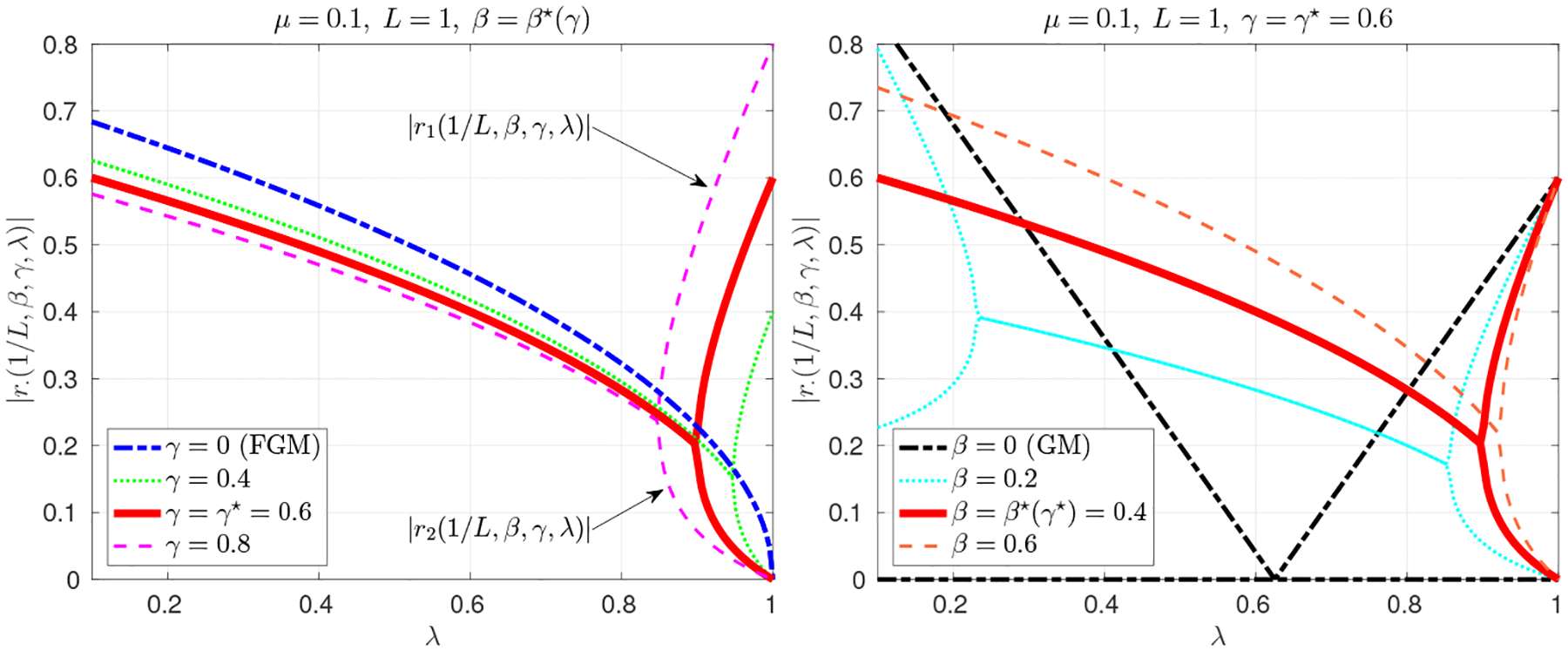
Plots of |r1(1/L, β, γ, λ)| and |r2(1/L, β, γ, λ)| over μ ≤ λ ≤ L for various (Left) γ values for given β = β⋆(γ), and (Right) β values for given γ = γ⋆, for a strongly convex quadratic problem with q = 0.1, where (β⋆, γ⋆) = (0.4, 0.6). Note that the maximum of |r1(1/L, β, γ, λ)| and |r2(1/L, β, γ, λ)|, i.e. the upper curve in the plot, corresponds to the value of ρ(Tλ(1/L, β, γ)) in (16).
Fig. 1 also illustrates spectral radius values for different choices of β for given γ = γ⋆, showing that suboptimal β value will slow down convergence. OGM with (α, β, γ) = (1/L, 0, γ) is equivalent to GM with , and Fig. 1 illustrates this choice for comparison. Interestingly, GM has some modes for mid-valued λ values that will converge faster than in the accelerated methods, but its overall convergence rate is worse. Apparently no one algorithm can have superior convergence rates for all modes.
Although using the optimized coefficients (β⋆, γ⋆) leads to OGM having the smallest possible overall spectral radius ρ(T(·)), the upper red and blue curves in Fig. 1 illustrate that this “tuned” OGM will have modes for large eigenvalues that converge slower than with OGM with γ = 0 (i.e., FGM). This behavior may be undesirable when such modes dominate the overall convergence behavior. Interestingly, Sec. 3.4 describes that the convergence of the primary sequence {yk} of OGM is not governed by such modes unlike the secondary sequence {xk} of OGM. Fig. 1 reveals change points across λ meaning that there are different regimes; Sec. 3.4 elaborates on this behavior building upon a dynamical system analysis of FGM [5, Sec. 4].
3.4. Convergence Properties of OGM When α = 1/L
[5, Sec. 4] analyzed a constant-step FGM as a linear dynamical system for minimizing a strongly convex quadratic function (11), and showed that there are three regimes of behavior for the system; low momentum, optimal momentum, and high momentum regimes. This section similarly analyzes OGM to better understand its convergence behavior when solving a strongly convex quadratic problem (11), complementing the previous section’s spectral radius analysis of OGM
We use the eigen-decomposition of Q = VΛV⊤ with Λ ≔ diag{λi}, where the eigenvalues {λi} are in an ascending order, i.e., μ = λ1 ≤ λ2 ≤ ⋯ ≤ λd = L. And for simplicity, we let p = 0 without loss of generality, leading to x* = 0. By defining and as the mode coefficients of the primary and secondary sequences respectively and using (12), we have the following d independently evolving identical recurrence relations for the evolution of w·,i and v·,i of the constant-step OGM respectively:
| (23) |
for i = 1, …, d, although the initial conditions differ as follows:
| (24) |
with w0,i = v0,i. The convergence behavior of the ith dynamical system of both w·,i and v·,i in (23) is determined by the characteristic polynomial (17) with and λ = λi. Unlike the previous sections that studied only the worst-case convergence performance using the largest absolute value of the roots of the polynomial (17), we next discuss the convergence behavior of OGM more comprehensively using (17) with and λ = λi for the cases where 1) λi = L and 2) λi < L.
1) λi = L: The characteristic polynomial (17) of the mode of λi = L reduces to r2 + γr = 0 with two roots 0 and −γ regardless of the choice of β. Thus we have monotone convergence for this (dth) mode of the dynamical system [21, Sec. 17.1]:
| (25) |
where cd and are constants depending on the initial conditions (24). Substituting w1,d = 0 and v1,d = −(β + γ)v0,d (24) into (23) yields cd = 0 and , illustrating that the primary sequence {wk,d} reaches its optimum after one iteration, whereas the secondary sequence {vk,d} has slow monotone convergence of the distance to the optimum, while exhibiting undesirable oscillation due to the term (−γ)k, corresponding to overshooting over the optimum.
2) λi < L: In (22) we found the optimal overall β⋆ for OGM. One can alternatively explore what the best value of β would be for any given mode of the system for comparison. The polynomial (17) has repeated roots for the following β, corresponding to the smaller zero of the discriminant Δ(1/L, β, γ, λi) for given γ and λi:
| (26) |
This root satisfies (22), because λ1 is the smallest eigenvalue. Next we examine the convergence behavior of OGM in the following three regimes, similar to FGM in [5, Sec. 4.3]:5
– : low momentum, over-damped,
– : optimal momentum, critically damped,
– : high momentum, under-damped.
If , the polynomial (17) has two real roots, r1,i and r2,i where we omit (1/L, β, γ, λi) in r·,i = r·(1/L, β, γ, λi) for simplicity. Then, the system evolves as [21, Sec. 17.1]:
| (27) |
where constants c1,i, c2,i, and depend on the initial conditions (24). In particular, when , we have the repeated root , corresponding to critical damping, yielding the fastest monotone convergence among (27) for any β s.t. . This property is due to the quasi-convexity of ρ(Tλ(1/L, β, γ)) over β. If , the system is over-damped, which corresponds to the low momentum regime, where the system is dominated by the larger root that is greater than , and thus has slow monotone convergence. However, depending on the initial conditions (24), the system may only be dominated by the smaller root, as noticed for the case λi = L in (25). Also note that the mode of λi = L is always in the low momentum regime regardless of the value of β.
If , the system is under-damped, which corresponds to the high momentum regime. This means that the system evolves as [21, Sec. 17.1]:
| (28) |
where the frequency of the oscillation is given by
| (29) |
and ci, δi, and denote constants that depend on the initial conditions (24); in particular for β ≈ 1, we have δi ≈ 0 and so we will ignore them.
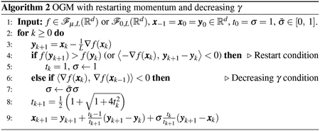
We categorize the behavior of the ith mode of OGM for each λi based on the above momentum analysis. Regimes with two curves and one curve in Fig. 1 correspond to the low- and high-momentum regimes, respectively. In particular, for β = β⋆(γ) in Fig. 1, most λi values experience high momentum (and the optimal momentum for λi satisfying , e.g., λi = μ), whereas modes where λi ≈ L experience low momentum. The fast convergence of the primary sequence {wk,d} in (25) generalizes to the case λi ≈ L, corresponding to the lower curves in Fig. 1. In addition, for β smaller than β⋆(γ) in Fig. 1, both λ ≈ μ and λ ≈ L experience low momentum so increasing β improves the convergence rate.
Based on the quadratic analysis, we would like to use appropriately large β and γ coefficients, namely (β⋆, γ⋆), to have fast monotone convergence (for the dominating modes). However, such values require knowing the function parameter q = μ/L that is usually unavailable in practice. Using OGM (with coefficients (7) and (9)) without knowing q will likely lead to oscillation due to the high momentum (or under-damping) for strongly convex functions. The next section describes restarting schemes inspired by [5] that we suggest to use with OGM to avoid such oscillation and thus heuristically accelerate the rate of OGM for a strongly convex quadratic function and even for a convex function that is locally well-conditioned.
4. Restarting Schemes
Restarting an algorithm (i.e., starting the algorithm again by using the current iterate as the new starting point) after a certain number of iterations or when some restarting condition is satisfied has been found useful, e.g., for the conjugate gradient method [22,23], called “fixed restart” and “adaptive restart” respectively. The fixed restart approach was also studied for accelerated gradient schemes such as FGM in [24, Sec. 11.4] [16]. Recently adaptive restart of FGM was shown to provide dramatic practical acceleration without requiring knowledge of function parameters [5,6,7]. Building upon those ideas, this section reviews and applies restarting approaches for OGM. A quadratic analysis in [5] justified using a restarting condition for FGM; this section extends that analysis to OGM by studying an observable quantity of oscillation that serves as an indicator for restarting the momentum of OGM.
4.1. Fixed Restart
Restarting an algorithm every k iterations can yield a linear rate for decreasing a function in [24, Sec. 11.4] [16, Sec. 5.1]. We examine this restart approach for OGM here. Let x j,i denote the jth outer iteration and ith inner iteration of an OGM variant that is restarted every k (inner) iterations. Specifically, this OGM uses x j+1,0 = x j,k to initialize the next (j + 1)th outer iteration. Combining the OGM bound (8) and the strong convexity inequality (2) yields the following linear rate of cost function decrease for k inner iterations of OGM:
| (30) |
This bound is smaller than the 4L/μk2 bound for FGM with fixed restart (using the FGM bound (4)). Here, an optimal restarting interval k that minimizes the bound (30) for a given total number of steps jk is .
There are two drawbacks of the fixed restart approach [5, Sec. 3.1]. First, computing the optimal interval kfixed requires knowledge of q that is usually unavailable in practice. Second, using a global parameters q may be too conservative when the iterates enter locally well-conditioned region. Therefore, adaptive restarting [5] has been found useful in practice, which we review next and then apply to OGM. The above two drawbacks also apply to the algorithms in Sec. 2 that assume knowledge of the global parameter q.
4.2. Adaptive Restart
To circumvent the drawbacks of fixed restart, [5] proposes the following two adaptive restart schemes for FGM:
- – Function scheme for restarting (FR): restart whenever
(31) - – Gradient scheme for restarting (GR): restart whenever
(32)
These schemes heuristically improve convergence rates of FGM with coefficients (3) and both performed similarly [5,7]. Although the function scheme guarantees monotonic decreasing function values, the gradient scheme has two advantages over the function scheme [5]; the gradient scheme involves only arithmetic operations with already computed quantities, and it is numerically more stable.
These two schemes encourage algorithm restart whenever the iterates take a “bad” direction, i.e., when the function value increases or the negative gradient and the momentum have an obtuse angle, respectively. However, a convergence proof that justifies their empirical acceleration is yet unknown, so [5] analyzes such restarting schemes for strongly convex quadratic functions. An alternative scheme in [7] that restarts whenever the magnitude of the momentum decreases, i.e., ∥yk+1 − yk∥ < ∥yk − yk−1∥, has a theoretical convergence analysis for the function class . However, empirically both the function and gradient schemes performed better in [7]. Thus, this paper focuses on adapting practical restart schemes to OGM and extending the analysis in [5] to OGM. First we introduce a new additional adaptive scheme designed specifically for OGM.
4.3. Adaptive Decrease of γ for OGM
Sec. 3.4 described that the secondary sequence {xk} of OGM might experience overshooting and thus slow convergence, unlike the primary sequence {yk}, when the iterates enter a region where the mode of the largest eigenvalue dominates. (Sec. 6.1.2 illustrates such an example.) From (25), the overshoot of xk has magnitude proportional to γ, yet a suitably large γ, such as γ⋆ (21), is essential for overall acceleration.
To avoid (or reduce) such overshooting, we suggest the following adaptive scheme:
- – Gradient scheme for decreasing γ (GDγ): decrease γ whenever
(33)
Because the primary sequence {yk} of OGM is unlikely to overshoot, one could choose to simply use the primary sequence {yk} as algorithm output instead of the secondary sequence {xk}. However, if one needs to use the secondary sequence of OGM (e.g., Sec. 5.2), adaptive scheme (33) can help.
4.4. Observable OGM Quantities
This section revisits Sec. 3.4 that suggested that observing the evolution of the mode coefficients {wk,i} and {vk,i} can help identify the momentum regime. However, in practice that evolution is unobservable because the optimum x* is unknown, whereas Sec. 3.4 assumed x* = 0. Instead we can observe the evolution of the function values, which are related to the mode coefficients as follows:
| (34) |
and also the inner products of the gradient and momentum, i.e.,
| (35) |
| (36) |
These quantities appear in the conditions for the adaptive schemes (31), (32), and (33).
One would like to increase β and γ as large as possible for acceleration up to β⋆ and γ⋆ (22). However, without knowing q (and β⋆, γ⋆), we could end up placing the majority of the modes in the high momentum regime, eventually leading to slow convergence with oscillation as described in Sec. 3.4. To avoid such oscillation, we hope to detect it using (34) and (35) and restart the algorithm. We also hope to detect the overshooting (25) of the modes of the large eigenvalues (in the low momentum regime) using (36) so that we can then decrease γ and avoid such overshooting.
We focus on the case where β > β1(γ) for given γ, when the most of the modes are in the high momentum regime. Because the maximum of ρ(Tλ(1/L, β, γ)) occurs at the points λ = μ or λ = L, we expect that (34), (35), and (36) will be quickly dominated by the mode of the smallest or the largest values. Using (25) and (28) leads to the following approximations:
| (37) |
where ψ1 = ψ1(β, γ). It is likely that these expressions will be dominated by the mode of either the smallest or largest eigenvalues. We next analyze each case separately.
4.4.1. Case 1: the Mode of the Smallest Eigenvalue Dominates
When the mode of the smallest eigenvalue dominates, we further approximate (37) as
| (38) |
using simple trigonometric identities and the approximations and sin(kψ1) ≈ sin((k + 1/2)ψ1). The values (38) exhibit oscillations at a frequency proportional to ψ1(β, γ) in (29). This oscillation can be detected by the conditions (31) and (32) and is useful in detecting the high momentum regime where a restart can help improve the convergence rate.
4.4.2. Case 2: the Mode of the Largest Eigenvalue Dominates
Unlike the primary sequence {yk} of OGM, convergence of the secondary sequence {xk} of OGM may be dominated by the mode of the largest eigenvalue in (25). By further approximating (37) for the case when the mode of the largest eigenvalue dominates, the function value decreases slowly but monotonically, whereas f(yk) ≈ f(x*) = 0 and 〈−∇f(xk), yk+1 − yk〉 ≈ 0. Therefore, neither restart condition (31) or (32) can detect such non-oscillatory observable values, even though the secondary mode {wk,d} of the largest eigenvalue is oscillating (corresponding to overshooting over the optimum). However, the inner product of two sequential gradients , can detect the overshoot of the secondary sequence {xk}, suggesting that the algorithm should adapt by decreasing γ when condition (33) holds. Decreasing γ too much may slow down the overall convergence rate when the mode of the smallest eigenvalue dominates. Thus, we use (33) only when using the secondary sequence of OGM as algorithm output (e.g., Sec. 5.2).
5. Proposed Adaptive Schemes for OGM
5.1. Adaptive Scheme of OGM for Smooth and Strongly Convex Problems
Alg. 2 illustrates a new adaptive version of OGM that is used in our numerical experiments in Sec. 6. When a restart condition is satisfied in Alg. 2, we reset tk = 1 to discard the previous momentum that has a bad direction. When the decreasing γ condition is satisfied in Alg. 2, we decrease σ to suppress undesirable overshoot of the secondary sequence {xk}. Although the analysis in Sec. 3 considered only strongly convex quadratic functions, the numerical experiments in Sec. 6 illustrate that the adaptive scheme is also useful more generally for smooth convex functions in , as described in [5, Sec. 4.6].
5.2. Adaptive Scheme of the Proximal Version of OGM for Nonsmooth Composite Convex Problems
Modern applications often involve nonsmooth composite convex problems:
| (39) |
where is a smooth convex function (typically not strongly convex) and is a convex function that is possibly nonsmooth and “proximal-friendly” [25], such as the ℓ1 regularizer ϕ(x) = ∥x∥1. Our numerical experiments in Sec. 6 show that a new adaptive version of a proximal variant of OGM can be useful for solving such problems.
To solve such problems using first-order information, [4] developed a fast proximal gradient method, popularized under the name fast iterative shrinkage-thresholding algorithm (FISTA), that directly extends FGM with coefficients (3) for solving (39) while preserving the O(1/k2) rate of FGM. Variants of FISTA with adaptive restart were studied in [5, Sec. 5.2].
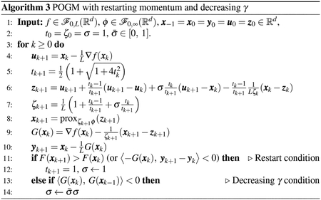
Inspired by the fact that OGM converges faster than FGM, [15] studied a proximal variant6 of OGM (POGM) with coefficients (7). It is natural to pursue acceleration of POGM by using variations of any (or all) of the three adaptive schemes (31), (32), (33), as illustrated in Alg. 3 where the proximity operator is defined as . As a function restart condition for POGM, we use F(xk+1) > F(xk) instead of F(yk+1) > F(yk), because F(yk) can be un-bounded (e.g., yk can be unfeasible for constrained problems). For gradient conditions of POGM, we consider the composite gradient mapping G(xk) in Alg. 3 that differs from the standard composite gradient mapping in [16]. We then use the gradient conditions 〈−G(xk), yk+1 − yk〉 < 0 and 〈G(xk), G(xk−1)〉 < 0 for restarting POGM or decreasing γ of POGM respectively. Here POGM must output the secondary sequence {xk} because the function value F(yk) of the primary sequence may be unbounded. This situation was the motivation for (33) (or 〈G(xk), G(xk−1)〉 < 0) and Sec. 4.3. When ϕ(x) = 0, Alg. 3 reduces to an algorithm that is similar to Alg. 2, where only the location of the restart and decreasing γ conditions differs.
The worst-case bound for POGM in [15] requires choosing the number of iterations N in advance for computing θN (7), which seems incompatible with adaptive restarting of POGM. Like (7) in Alg. 1, the fact that θN (7) is larger than the standard tN in (9) at the last iteration helps to dampen (by reducing the values of β and γ) the final update to guarantee fast convergence in the worst-case. (This property was studied for smooth convex minimization in [14].) We could perform one last update using θN after a restart condition is satisfied, but this step appears unnecessary because restarting already has the effect of slowing down the algorithm. Thus, we did not include any such extra update in Alg. 3 in our experiment in the next section.
6. Numerical Results
This section shows the results of applying OGM (and POGM) with adaptive schemes to various numerical examples including both strongly convex quadratic problems and non-strongly convex problems.7 The results illustrate that OGM (or POGM) with adaptive schemes converges faster than FGM (or FISTA) with adaptive restart. The plots show the decrease of F(yk) of the primary sequence for FGM (FISTA) and OGM unless specified. For POGM, we use the secondary sequence {xk} as an output and plot F(xk), since F(yk) can be unbounded.
6.1. Strongly Convex Quadratic Examples
This section considers two types of strongly convex quadratic examples, where the mode of either the smallest eigenvalue or the largest eigenvalue dominates, providing examples of the analysis in Sec. 4.4.1 and 4.4.2 respectively.
6.1.1. Case 1: the Mode of the Smallest Eigenvalue Dominates
Fig. 2 compares GM, FGM and OGM, with or without the knowledge of q, for minimizing a strongly convex quadratic function (11) in d = 500 dimensions with q = 10−4, where we generated A (for Q = A⊤A) and p randomly. In Fig. 2, ‘GM’ and ‘GM-q’ denote GM with and respectively. ‘FGM’ and ‘FGM-q’ denote step coefficients (3) and (5) respectively. ‘OGM’ and ‘OGM-q’ denote step coefficients (9) and (22) respectively. As expected, knowing q accelerates convergence.
Fig. 2.
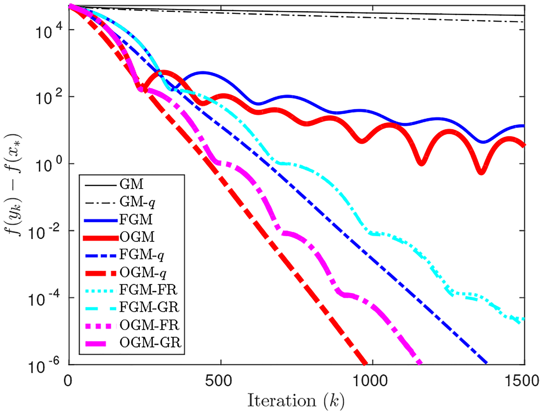
Minimizing a strongly convex quadratic function - Case 1: the mode of the smallest eigenvalue dominates. (FGM-FR and FGM-GR are almost indistinguishable, as are OGM-FR and OGM-GR.)
Fig. 2 also illustrates that adaptive restart helps FGM and OGM to nearly achieve the fast linear converge rate of their non-adaptive versions that know q. As expected, OGM converges faster than FGM for all cases. In Fig. 2, ‘FR’ and ‘GR’ stand for function restart (31) and gradient restart (32), respectively, and both behave nearly the same.
6.1.2. Case 2: the Mode of the Largest Eigenvalue Dominates
Consider the strongly convex quadratic function with , q = 0.01, p = 0 and x* = 0. When starting the algorithm from the initial point {x0} = (0.2, 1), the secondary sequence {xk} of OGM-GR8 (or equivalently OGM-GR-GDγ ) is dominated by the mode of largest eigenvalue in Fig. 3, illustrating the analysis of Sec. 4.4.2. Fig. 3 illustrates that the primary sequence of OGM-GR converges faster than that of FGM-GR, whereas the secondary sequence of OGM-GR initially converges even slower than GM. To deal with such slow convergence coming from the overshooting behavior of the mode of the largest eigenvalue of the secondary sequence of OGM, we employ the decreasing γ scheme in (33). Fig. 3 shows that using in Alg. 2 leads to overall faster convergence of the secondary sequence {xk} than the standard OGM-GR where . We leave optimizing the choice of or studying other strategies for decreasing γ as future work.
Fig. 3.
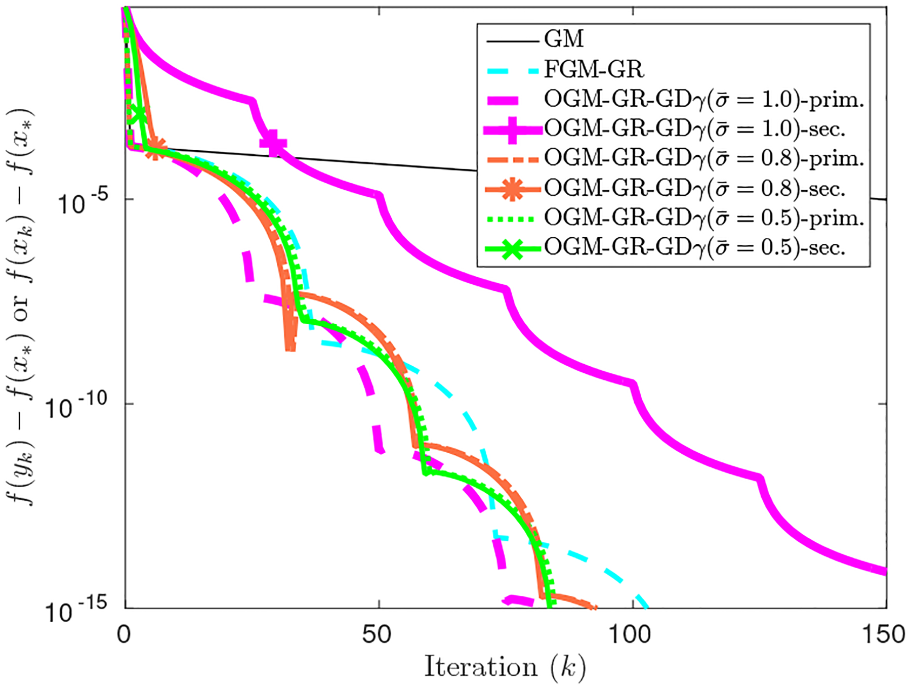
Minimizing a strongly convex quadratic function - Case 2: the mode of the largest eigenvalue dominates for the secondary sequence {xk} of OGM. Using GDγ (33) with accelerates convergence of the secondary sequence of OGM-GR, where both the primary and secondary sequences behave similarly after first few iterations, unlike .
6.2. Non-strongly Convex Examples
This section applies adaptive OGM (or POGM) to three non-strongly convex numerical examples in [5, 7]. The numerical results show that adaptive OGM (or POGM) converges faster than FGM (or FISTA) with adaptive restart.
6.2.1. Log-Sum-Exp
The following function from [5] is smooth but non-strongly convex:
It approaches as η → 0. Here, η controls the function smoothness where . The region around the optimum is approximately quadratic since the function is smooth, and thus the adaptive restart can be useful without knowing the local condition number.
For (m, d) = (100, 20), we randomly generated and for i = 1, …, m, and investigated η = 1, 10. Fig. 4 shows that OGM with adaptive restart converges faster than FGM with the adaptive restart. The benefit of adaptive restart is dramatic here; apparently FGM and OGM enter a locally well-conditioned region after about 100 − 200 iterations, where adaptive restart then provide a fast linear rate.
Fig. 4.
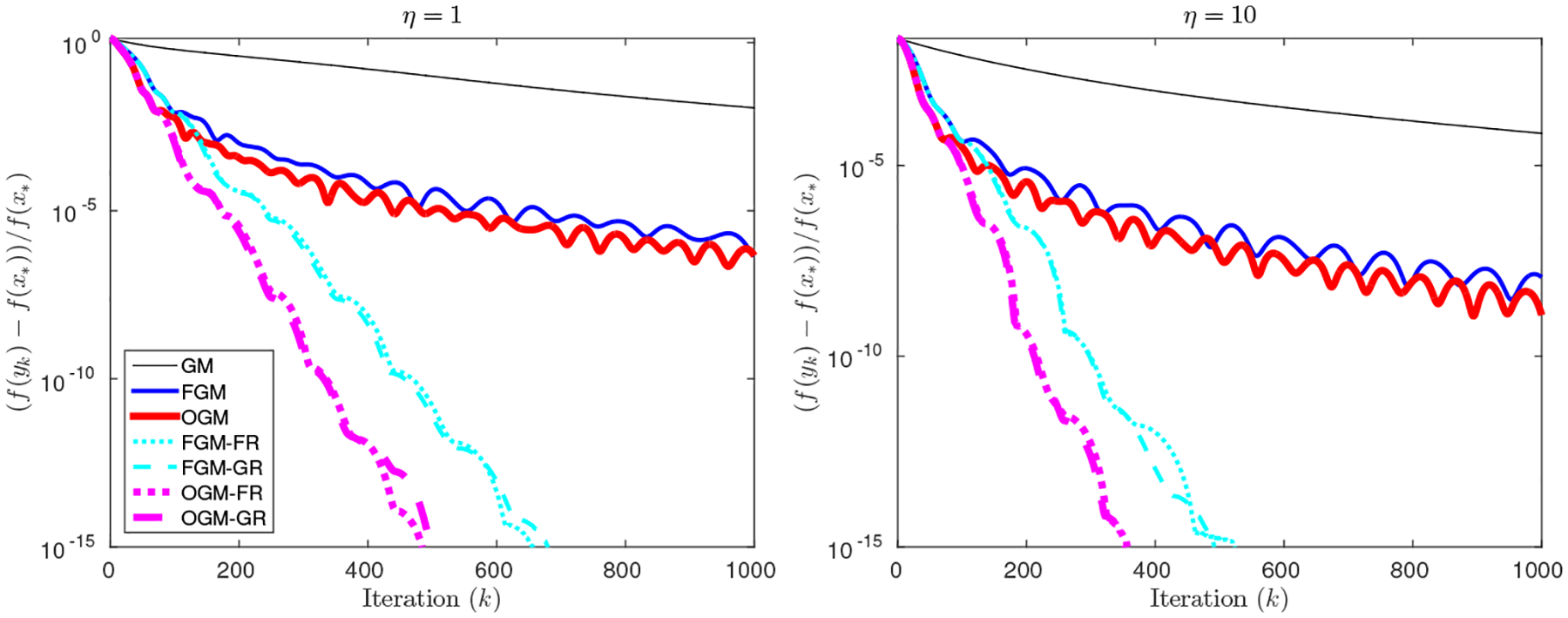
Minimizing a smooth but non-strongly convex Log-Sum-Exp function.
6.2.2. Sparse Linear Regression
Consider the following cost function used for sparse linear regression:
for , where L = λmax(A⊤A) and the parameter τ balances between the measurement error and signal sparsity. The proximity operator becomes a soft-thresholding operator, e.g., . The minimization seeks a sparse solution x*, and often the cost function is strongly convex with respect to the non-zero elements of x*. Thus we expect to benefit from adaptive restarting.
For each choice of (m, d, s, τ) in Fig. 5, we generated an s-sparse true vector xtrue by taking the s largest entries of a randomly generated vector. We then simulated b = Axtrue + ε, where the entries of matrix A and vector ε were sampled from a zero-mean normal distribution with variances 1 and 0.1 respectively. Fig. 5 illustrates that POGM with adaptive schemes provide acceleration over FISTA with adaptive restart. While Sec. 3.4 discussed the undesirable overshooting behavior that a secondary sequence of OGM (or POGM) may encounter, these examples rarely encountered such behavior. Therefore the choice of in the adaptive POGM was not significant in this experiment, unlike Sec. 6.1.2.
Fig. 5.
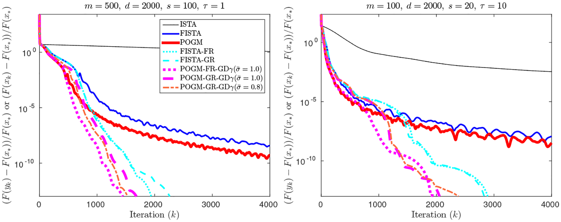
Solving a sparse linear regression problem. (ISTA is a proximal variant of GM.)
6.2.3. Constrained Quadratic Programming
Consider the following box-constrained quadratic program:
where L = λmax(Q). The algorithms ISTA (a proximal variant of GM), FISTA and POGM use the projection operator: . Fig. 6 denotes each algorithm by a projected GM, a projected FGM, and a projected OGM respectively. Similar to Sec. 6.2.2, after the algorithm identifies the active constraints the problem typically becomes a strongly convex quadratic problem where we expect to benefit from adaptive restart.
Fig. 6.
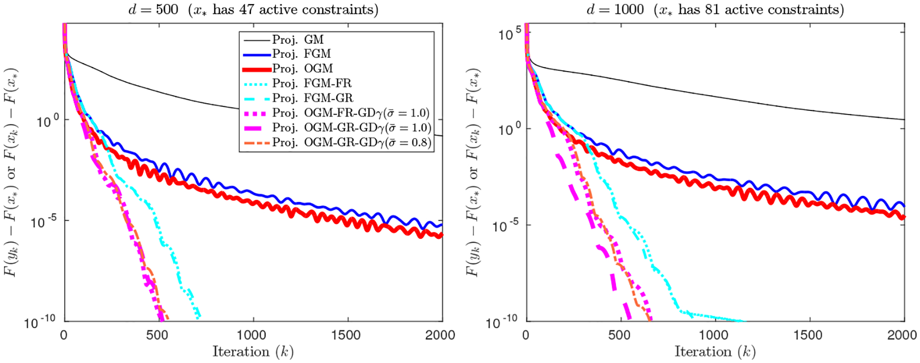
Solving a box-constrained quadratic programming problem.
Fig. 6 studies two examples with problem dimensions d = 500, 1000, where we randomly generate a positive definite matrix Q having a condition number 107 (i.e., q = 10−7), and a vector p. Vectors l and u correspond to the interval constraints −1 ≤ xi ≤ 1 for x = {xi}. The optimum x* had 47 and 81 active constraints out of 500 and 1000 respectively. In Fig. 6, the projected OGM with adaptive schemes converged faster than FGM with adaptive restart and other non-adaptive algorithms.
7. Conclusions
We introduced adaptive restarting schemes for the optimized gradient method (OGM) that heuristically exhibits a fast linear convergence rate when the function is strongly convex or even when the function is not globally strongly convex. The method resets the momentum when it makes a bad direction. We provided a heuristic dynamical system analysis to justify the practical acceleration of the adaptive scheme of OGM, by extending the existing analysis of FGM. On the way, we described new optimized constant step coefficients for OGM for strongly convex quadratic problems. Numerical results illustrate that the proposed adaptive approach practically accelerates the convergence rate of OGM, and in particular, performs faster than FGM with adaptive restart. An interesting open problem is to determine the worst-case bounds for OGM (and FGM) with adaptive restart.
Acknowledgements
This research was supported in part by NIH grant U01 EB018753.
Footnotes
For some applications even estimating L is expensive, and one must employ a backtracking scheme [4] or similar approaches. We assume L is known throughout this paper. An estimate of μ could be found by a backtracking scheme as described in [16, Sec. 5.3].
Very recently, [18] developed a new first-order method with known q that achieves a linear convergence rate for the cost function decrease that is faster than the linear rate in (6) for FGM.
It is straightforward to show that ρ(Tλ(α, β, γ)) in (16) is quasi-convex over λ. First, is quasi-convex over λ (for Δ(α, β, γ, λ) < 0). Second, the eigenvalue λ satisfying Δ(α, β, γ, λ) ≥ 0 is in the region where the function either monotonically increases or decreases, which overall makes the continuous function ρ(Tλ(α, β, γ)) quasi-convex over λ. This proof can be simply applied to other variables, i.e., ρ(Tλ(α, β, γ)) is quasi-convex over either α, β or γ.
For FGM with (5), the value of ρ(TL(1/L, β, 0)) is 0, and the function ρ(Tμ(1/L, β, 0)) is continuous and quasi-convex over β (see footnote 3). The minimum of ρ(Tμ(1/L, β, 0)) occurs at the point in (5) satisfying Δ(1/L, β, 0, μ) = 0, verifying the statement that FGM with (5) results from optimizing (18) over β given and γ = 0.
For simplicity in the momentum analysis, we restricted the choice of β within [0 1], containing the βk values of FGM in (3), (5) and OGM in (7), (9). This restriction simply discards the effect of a larger solution β of Δ(1/L, β, γ, λi) = 0 in the analysis, which is larger than 1.
Applying the proximity operator to the primary sequence {yk} of OGM, similar to the extension of FGM to FISTA, leads to a poor worst-case convergence bound [15]. Therefore, [15] applied the proximity operator to the secondary sequence of OGM and showed numerically that this version has a convergence bound about twice smaller than that of FISTA.
Software for the algorithms and for producing the figures in Sec. 6 is available at https://gitlab.eecs.umich.edu/michigan-fast-optimization/ogm-adaptive-restart.
Fig. 3 only compares the results of the gradient restart (GR) scheme for simplicity, where the function restart (FR) behaves similarly.
References
- 1.Cevher V, Becker S, Schmidt M: Convex optimization for big data: scalable, randomized, and parallel algorithms for big data analytics. IEEE Sig. Proc. Mag 31(5), 32–43 (2014) [Google Scholar]
- 2.Nesterov Y: A method for unconstrained convex minimization problem with the rate of convergence O(1/k2). Dokl. Akad. Nauk. USSR 269(3), 543–7 (1983) [Google Scholar]
- 3.Nesterov Y: Introductory lectures on convex optimization: A basic course. Kluwer; (2004) [Google Scholar]
- 4.Beck A, Teboulle M: A fast iterative shrinkage-thresholding algorithm for linear inverse problems. SIAM J. Imaging Sci 2(1), 183–202 (2009) [Google Scholar]
- 5.O’Donoghue B, Candès E: Adaptive restart for accelerated gradient schemes. Found. Comp. Math 15(3), 715–32 (2015) [Google Scholar]
- 6.Giselsson P, Boyd S: Monotonicity and restart in fast gradient methods. In: Proc. Conf. Decision and Control, pp. 5058–63 (2014) [Google Scholar]
- 7.Su W, Boyd S, Candès EJ: A differential equation for modeling Nesterov’s accelerated gradient method: theory and insights. J. Mach. Learning Res 17(153), 1–43 (2016) [Google Scholar]
- 8.Muckley MJ, Noll DC, Fessler JA: Fast parallel MR image reconstruction via B1-based, adaptive restart, iterative soft thresholding algorithms (BARISTA). IEEE Trans. Med. Imag 34(2), 578–88 (2015) [DOI] [PMC free article] [PubMed] [Google Scholar]
- 9.Monteiro RDC, Ortiz C, Svaiter BF: An adaptive accelerated first-order method for convex optimization. Comput. Optim. Appl 64(1), 31–73 (2016) [Google Scholar]
- 10.Kim D, Fessler JA: Optimized first-order methods for smooth convex minimization. Mathematical Programming 159(1), 81–107 (2016) [DOI] [PMC free article] [PubMed] [Google Scholar]
- 11.Drori Y, Teboulle M: Performance of first-order methods for smooth convex minimization: A novel approach. Mathematical Programming 145(1–2), 451–82 (2014) [Google Scholar]
- 12.Drori Y: The exact information-based complexity of smooth convex minimization. J. Complexity 39, 1–16 (2017) [Google Scholar]
- 13.Kim D, Fessler JA: Generalizing the optimized gradient method for smooth convex minimization (2016). Arxiv 1607.06764
- 14.Kim D, Fessler JA: On the convergence analysis of the optimized gradient method. J. Optim. Theory Appl 172(1), 187–205 (2017) [DOI] [PMC free article] [PubMed] [Google Scholar]
- 15.Taylor AB, Hendrickx JM, Glineur François.: Exact worst-case performance of first-order algorithms for composite convex optimization (2015). Arxiv 1512.07516
- 16.Nesterov Y: Gradient methods for minimizing composite functions. Mathematical Programming 140(1), 125–61 (2013) [Google Scholar]
- 17.Güler O: New proximal point algorithms for convex minimization. SIAM J. Optim 2(4), 649–64 (1992) [Google Scholar]
- 18.Van Scoy B, Freeman RA, Lynch KM: The fastest known globally convergent first-order method for the minimization of strongly convex functions (2017). URL http://www.optimization-online.org/DB_HTML/2017/03/5908.html
- 19.Polyak BT: Introduction to optimization. Optimization Software Inc, New York: (1987) [Google Scholar]
- 20.Lessard L, Recht B, Packard A: Analysis and design of optimization algorithms via integral quadratic constraints. SIAM J. Optim 26(1), 57–95 (2016) [Google Scholar]
- 21.Chiang A: Fundamental methods of mathematical economics. McGraw-Hill, New York: (1984) [Google Scholar]
- 22.Powell MJD: Restart procedures for the conjugate gradient method. Mathematical Programming 12(1), 241–54 (1977) [Google Scholar]
- 23.Nocedal J, Wright SJ: Numerical optimization. Springer, New York: (2006). DOI 10.1007/978-0-387-40065-5. 2nd edition. [DOI] [Google Scholar]
- 24.Nemirovski A: Efficient methods in convex programming (1994). URL http://www2.isye.gatech.edu/~nemirovs/Lect_EMCO.pdf. Lecture notes
- 25.Combettes PL, Pesquet JC: Proximal splitting methods in signal processing (2011). DOI 10.1007/978-1-4419-9569-8_10. Fixed-Point Algorithms for Inverse Problems in Science and Engineering, Springer, Optimization and Its Applications, pp 185–212 [DOI] [Google Scholar]


