QED limits for many-server systems under a priority policy

Abstract

A multi-class many-server priority system operating in the quality-and-efficiency-driven regime is considered. Both arrival processes and service times are general. The many-server heavy-traffic diffusion asymptotic is characterized in terms of the corresponding limiting infinite-server process.

Appendices

Proofs

1.1 Proof of Lemma 1

For $l=1,\dots ,k$, one has

(46)

where $\hat{B}^n_l:=\{\hat{B}^n_l(t),\; t\ge 0\}$ is a centered random walk:

$$\begin{aligned} \hat{B}^n_l(t):=\frac{1}{\sqrt{n}}\sum _{j=1}^{\lfloor nt\rfloor }\left( {1}_{\{s_{l,j}>0\}}-\bar{G}_l(0)\right) . \end{aligned}$$

Then, we have, as $n\rightarrow \infty$,

$$\begin{aligned} (\hat{B}^n_1,\dots , \hat{B}^n_k) \Rightarrow (B_1,\dots , B_k) . \end{aligned}$$

(47)

In addition, continuity of $(x_1,\dots ,x_k)\mapsto (\bar{G}_1(0)x_1,\dots \bar{G}_k(0)x_k)$, the continuous mapping theorem and (4) yield, as $n\rightarrow \infty$,

$$\begin{aligned} (\bar{G}_1(0)\hat{A}^n_1,\dots ,\bar{G}_k(0)\hat{A}^n_k)\Rightarrow (\bar{G}_1(0)\hat{A}_1,\dots ,\bar{G}_k(0)\hat{A}_k). \end{aligned}$$

(48)

Furthermore, $E^n_l=A^n_l+\kappa _l^n$, (4) and (10) imply, as $n\rightarrow \infty$,

$$\begin{aligned} n^{-1}\left( {E^n_1},\dots ,{E^n_k}\right) \Rightarrow \left( \lambda _1e,\dots ,\lambda _ke\right) \quad \text {and} \quad n^{-1}\left( {\kappa ^n_1},\dots ,{\kappa ^n_k}\right) \Rightarrow (0,\dots ,0). \end{aligned}$$

Finally, the lemma follows from (46)–(48), the last two limits and $\lambda _l=0$, $l>k^\star$; by definition, the $\hat{B}^n_l$ are mutually independent, as well as independent of $(\hat{A}^n_1,\dots , \hat{A}^n_k)$.

1.2 Proof of Lemma 2

In view of

continuity of $(x,x_1,\dots ,x_k)\mapsto (x-\sum _ {l=1}^k G_l(0)x_l, \bar{G}_1(0)x_1,\dots ,\bar{G}_k(0)x_k)$ and (10), it is enough to show, for $l=1,\dots ,k$,

as $n\rightarrow \infty$. To this end, one has, for $\varepsilon >0$ and b (that is a continuity point of the distribution of $\hat{\kappa }_l$),

$$\begin{aligned}&\mathbb {P}\left[ \left| \frac{1}{\sqrt{n}}\sum _{j=1}^{\kappa ^n_l}\left( {1}_{\{s_{l,j}>0\}}-\bar{G}_l(0)\right) \right|>\varepsilon \right] \\&\quad \le \mathbb {P}\left[ \sup _{c\le b}\left| \frac{1}{\sqrt{n}}\sum _{j=1}^{\lfloor \sqrt{n}c\rfloor }\left( {1}_{\{s_{l,j}>0\}}-\bar{G}_l(0)\right) \right|>\varepsilon \right] +\mathbb {P}\left[ \hat{\kappa }^n_l>b\right] \\&\quad \rightarrow \mathbb {P}\left[ \hat{\kappa }_l>b\right] , \end{aligned}$$

as $n\rightarrow \infty$; the limit follows from a SLLN (for example, see [11]) and (10). By selecting a high enough value of b, the right-hand side can be made arbitrarily small. Hence, the lemma holds.

1.3 Proof of Lemma 3

Straightforward algebra yields, for $t \ge 0$,

$$\begin{aligned} \nonumber \hat{Z}^n(t)&= \beta ^n \bar{\ddot{G}}^n(t) - \left( \hat{\xi }^n\right) ^-\bar{\ddot{G}}^n(t)+\sum _{l=1}^k \hat{\kappa }^n_l\bar{ G}_l(t) + \sum _{l=1}^k\int _{0}^t\bar{G}_l(t-s)\, \hat{A}^n_l(\mathrm ds) \\&\qquad +\,\frac{1}{\sqrt{n}}\sum _{l=1}^{k}\sum _{j=1}^{E^n_l(t)}\left( {1}_{\{s_{l,j}+\tau _{l,j}>t\}}-\bar{G}_l(t-\tau _{l,j})\right) +\frac{1}{\sqrt{n}}\sum _{j=1}^{\xi ^n\wedge n}\left( {1}_{\{\ddot{s}_{j}>t\}}-\bar{\ddot{G}}^n(t) \right) . \end{aligned}$$

(49)

Next, we consider the elements on the right-hand side of (49). First, (6), (9) and (10) result in, as $n\rightarrow \infty$,

$$\begin{aligned} \beta ^n\bar{\ddot{G}}^n-\left( \hat{\xi }^n\right) ^-\bar{\ddot{G}}^n+\sum _{l=1}^k \hat{\kappa }^n_l\bar{ G}_l\Rightarrow \beta \bar{\ddot{G}}-\hat{\xi }^-\bar{\ddot{G}}+\sum _{l=k^\star }^k\hat{\kappa }_l\bar{G}_l. \end{aligned}$$

(50)

Second, (4) implies, as $n\rightarrow \infty$,

$$\begin{aligned} \left\{ \sum _{l=1}^{k} \int _0^t\bar{G}_l(t-s) \, \hat{A}^n(\mathrm ds),\, t\ge 0 \right\} \Rightarrow \left\{ \sum _{l=1}^{k} \int _0^t\bar{G}_l(t-s) \, \hat{A}(\mathrm ds),\, t\ge 0 \right\} . \end{aligned}$$

(51)

Third, let $\breve{M}_l^n:=\{\breve{M}^n_l(t),\; t\ge 0\}$, where

$$\begin{aligned} \breve{M}^n_l(t) :=\frac{1}{\sqrt{n}}\sum _{j=1}^{E^n_l(t)}\left( {1}_{\{s_{l,j}+\tau _{l,j}>t\}}-\bar{G}_l(t-\tau _{l,j})\right) ; \end{aligned}$$

furthermore, define $M^n_l:=\{M^n_l(t), \; t\ge 0\}$, where

$$\begin{aligned} M^n_l(t):=\frac{1}{\sqrt{n}}\sum _{j=1}^{\lfloor {\lambda }^n_lt\rfloor }\left( {1}_{\{{s}_{l,j}+j/\lambda ^n_l>t\}}-\bar{{G}}_l(t - j/\lambda ^n_l)\right) . \end{aligned}$$

By following the steps outlined in the proof of [31, Lemma 3], one can show $(\breve{M}^n_l, M^n_l)\Rightarrow (M_l,M_l)$, as $n\rightarrow \infty$, where $M_l:=\{M_l(t),\; t\ge 0\}$ is a centered Gaussian process with a.s. continuous paths, $M_l(0)=0$ and

$$\begin{aligned} \mathbb {E}M_l(t)M_l(t+\delta )=\lambda _l\int _0^t\bar{G}_l(t+\delta -u)G_l(t-u) \, \mathrm du, \ \ \ \delta \ge 0. \end{aligned}$$

Since $\{M^n_l, \;l=1,\dots , k\}$ are independent, $\{M_l,\; l=1,\dots , k\}$ are independent as well. Therefore, we have, as $n\rightarrow \infty$,

$$\begin{aligned} \breve{M}^n_{1:k} \Rightarrow M. \end{aligned}$$

(52)

Fourth, let $\hat{U}^n:=\{\hat{U}^n(t,s), t\ge 0,\, 0\le s\le 1\}$, where

$$\begin{aligned} \hat{U}^n(t,s)= \frac{1}{\sqrt{n}}\sum _{j=1}^{\lfloor nt\rfloor }\left( {1}_{\{\eta _j\le s\}}-s\right) , \end{aligned}$$

and $\{\eta _j,\; j\ge 1\}$ is a sequence of independent [0, 1]-uniform random variables. Then, the last term in (49) can be expressed in terms of $\hat{U}^n$:

$$\begin{aligned} \frac{1}{\sqrt{n}}\sum _{j=1}^{\xi ^n\wedge n}\left( {1}_{\{\ddot{s}_{j}>t\}}-\bar{\ddot{G}}^n(t) \right) =\hat{U}^n(n^{-1} \xi ^n\wedge 1, \, \ddot{G}^n(t)). \end{aligned}$$

Now, $\hat{U}^n\Rightarrow \hat{U}$, as $n\rightarrow \infty$, where $\hat{U}$ is a Kiefer process [25, Lemma 3.1]. The last limit, together with continuity of $\hat{U}$, (9) and (10), yields, as $n\rightarrow \infty$,

$$\begin{aligned} \left( \hat{U}^n(n^{-1}\xi ^n\wedge 1, \ddot{G}^n), \, \hat{U}^n(1, \ddot{G}^n)\right) \Rightarrow (V\circ \ddot{G}, \, V\circ \ddot{G}), \end{aligned}$$

(53)

where V is as in the statement of the lemma.

Finally, the statement of the lemma follows from (50)–(53). All limiting terms have a.s. continuous paths, except possibly $\sum _{l=k^\star }^k\hat{\kappa }_l\bar{G}_l$. Independence of the limiting terms is due to independence of $\xi ^n$, $M^n_{1:k}$ (rather than $\breve{M}^n_{1:k}$), $\{A^n_{l},\; l=1,\dots ,k\}$ and $\hat{U}^n(1, \ddot{G}^n)$ (rather than $\hat{U}^n(n^{-1} \xi ^n\wedge 1,\, \ddot{G}^n)$).

1.4 Proof of Lemma 4

Note that

holds for $l=1,\dots , k$. Utilizing the preceding equality twice (for l and k), and combining it with (3) results in

(54)

In addition, priority of class-i customers over class-j ($j>i$) customers implies

(55)

on the left-hand side is the event that throughout the time interval [u, t] at least one class-i ($1 \le i \le l$) customer awaits service, and on the right-hand side is the event that no class-j ($l+1 \le j \le k$) customer enters service in the time interval [u, t].

Next, (54) and (55) are used to prove the statement of the lemma. To this end, let . Then, two cases are of interest:

• $u_t=\infty$: It follows that , and hence for any $u \le t$. This, together with (54) and nonnegativity of the double sum in (54), results in

  

  for $u \le t$. Therefore, the supremum in the statement of lemma is non-positive, and the lemma holds in this case.

• $0 \le u_t \le t$: It follows that (also in the case when $u_t=0$, due to our notation) and $0$ for $u \in [u_t,t]$. Then, (54) and (55) imply that, for $u \in [0,t]$,

  

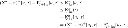
  Hence, the lemma holds in this case as well.

This completes the proof.

Ancillary results

Lemma 7

Let $f_i:D[0,\infty ) \rightarrow D[0,\infty )$, $i=1,\dots ,k$, be measurable and Lipschitz continuous with Lipschitz constant $c_i$, such that $f_i(0)=0$. If $z \in D[0,\infty )$, then:

• (i) The mapping $g_z: \, D[0,\infty ) \rightarrow D[0,\infty )$ defined by

  $$\begin{aligned} g_z(x)(t):=z(t)+\sum _{l=1}^{k}\int _0^t f_l(x)(t-s) \, G_l(\mathrm ds) \end{aligned}$$

  is $J_1$-measurable and Lipschitz continuous in $(D[0,\infty ),\Vert \cdot \Vert )$.

Furthermore, if $G_\vee (0):= \vee _{l=1}^k G_l(0) =0$, then the following hold:

• (ii) The equation $x=g_z(x)$ has a unique solution in $D[0,\infty )$.

• (iii) The mapping $g:D[0,\infty ) \rightarrow D[0,\infty )$, defined such that g(z) is the unique solution of $x=g_z(x)$, is $J_1$-measurable and Lipschitz continuous in $(D[0,\infty ),\Vert \cdot \Vert )$.

• (iv) Define $x_{i+1}:=g_z(x_{i})$, $i\ge 0$, where $x_0 \in D[0,\infty )$ is given. Then $x_i\rightarrow g(z)$, as $i\rightarrow \infty$. Moreover, for any $t\ge 0$, there exist an $i_0>0$ (a function of $G_\vee$) and $c>0$ (a function of $G_\vee$ and $c_{1:k}$) such that, for $i\ge i_0$,

  $$\begin{aligned} \Vert x_i-g(z)\Vert _t\le c \left( \frac{c_{1:k}}{c_{1:k}+1}\right) ^i(\Vert z-x_0\Vert _t+\Vert x_0\Vert _t). \end{aligned}$$

Remark 6

The assumption $G_\vee (0)=0$ is essential. Without this assumption, there exist examples that demonstrate that the lemma does not hold.

Proof

Part (i) For $t\ge 0$, one has

$$\begin{aligned} |g_z(x_1)(t)-g_z(x_2)(t)|&\le \sum _{l=1}^{k}\int _0^t |f_l(x_1)-f_l(x_2)|(t-s) \, G_l(\mathrm ds) \nonumber \\&\le \sum _{l=1}^k\int _0^t c_l\Vert x_1-x_2\Vert _{t-s} \, G_l(\mathrm ds) \nonumber \\&\le \Vert x_1-x_2\Vert _{t}\sum _{l=1}^k c_l G_l(t), \end{aligned}$$

(56)

and therefore

$$\begin{aligned} \Vert g_z(x_1)-g_z(x_2)\Vert _t \le c_{1:k} \Vert x_1-x_2\Vert _t. \end{aligned}$$

(57)

The proof of measurability follows from measurability of $x\mapsto y$, where $y(t):=\int _0^t x^+(t-s)\, G_l(\mathrm ds)$ for $l=1,\dots ,k$ (see the proof of Proposition 3.1 in [34]), the fact that the $f_l$ are measurable functions, and the fact that compositions and sums of measurable functions are measurable.

Part (ii) We argue the uniqueness first. Suppose $x,y\in D[0,T]$ such that $x = g_z(x)$ and $y = g_z(y)$. Since $G_\vee (0)=0$, there exists a $\delta >0$ such that $G_\vee (\delta )<(c_{1:k}+1)^{-1}$. Then, (56) implies

$$\begin{aligned} \Vert x-y\Vert _{\delta }=\Vert g_z(x)-g_z(y)\Vert _{\delta }\le \Vert x-y\Vert _{\delta }\frac{c_{1:k}}{c_{1:k}+1}, \end{aligned}$$

which yields $\Vert x-y\Vert _{\delta }=0$. Next, suppose $\Vert x-y\Vert _{(i-1)\delta }=0$ for some $i>2$ (the induction hypothesis). Then, for $t\in ((i-1)\delta ,i\delta ]$, one has

$$\begin{aligned} |x(t)-y(t)|&=|g_z(x)(t)-g_z(y)(t)| \\&\le \sum _{l=1}^{k}\int _0^t \Vert f_l(x)-f_l(y)\Vert _{t-s} \, G_l(\mathrm ds)\\&\le \sum _{l=1}^k\int _{0}^\delta c_l\Vert x-y\Vert _{i\delta } \, G_l(\mathrm ds) \\&\le \Vert x-y\Vert _{i\delta } \frac{c_{1:k}}{c_{1:k}+1}; \end{aligned}$$

the second inequality follows from the induction hypothesis, while the last inequality follows from definition of $\delta$. Combining the last relationship and $\Vert x-y\Vert _{(i-1)\delta }=0$ results in

$$\begin{aligned} \Vert x-y\Vert _{i\delta }\le \Vert x-y\Vert _{i\delta } \frac{c_{1:k}}{c_{1:k}+1}, \end{aligned}$$

which yields $\Vert x-y\Vert _{i\delta }=0$. Hence, the uniqueness follows.

Now, we demonstrate that there exists a solution. Define the sequence $\{x_i, \, i\ge 0\}$: $x_{i+1}=g_z(x_i)$, $i\ge 0$, for a given $x_0\in D[0,\infty )$. We argue that $\{x_i, \, i\ge 0\}$ is a Cauchy sequence. First, we prove by induction that, for $t\ge 0$ and $i \ge 1$,

$$\begin{aligned} \Vert x_{i+1} - x_i \Vert _t \le (c_{1:k} +1) \, c_{1:k}^i \, (\Vert z -x_0 \Vert _t + \Vert x_0 \Vert _t) \, G^{(i)}_\vee (t), \end{aligned}$$

(58)

where $G^{(i)}_\vee$ denotes the i-fold convolution of $G_\vee$ with itself. The base ($i=0$) of the induction can be verified as follows:

$$\begin{aligned} |x_1(t) - x_0(t)|&\le |z(t) - x_0(t)| + \sum _{l=1}^k\int _0^t \Vert f_l(x_0) \Vert _{t-s} \, G_l(\mathrm ds) \\&\le \Vert z-x_0\Vert _t + c_{1:k}\Vert x_0\Vert _t \\&\le ( c_{1:k} +1)\left( \Vert z-x_0\Vert _t+\Vert x_0\Vert _t\right) , \end{aligned}$$

and, thus, $\Vert x_1-x_0\Vert _t\le ( c_{1:k} +1 )\left( \Vert z-x_0\Vert _t+\Vert x_0\Vert _t\right)$. Assuming that (58) holds for some $i=j-1$ yields that (58) holds for $i=j$ as well:

$$\begin{aligned} |x_{j+1}(t)-x_j(t)|&\le \sum _{l=1}^k \int _0^t \Vert f_l(x_j)-f_l(x_{j-1})\Vert _{t-s} \, G_l(\mathrm ds)\\&\le (c_{1:k} +1) \, c_{1:k}^j \, (\Vert z-x_0\Vert _t +\Vert x_0\Vert _t) \, \int _0^t G_\vee ^{(j-1)}(t-s) \, G_\vee (\mathrm ds) \\&\le (c_{1:k} +1) \, c_{1:k}^j \, (\Vert z-x_0\Vert _t +\Vert x_0\Vert _t) \, G_\vee ^{(j)}(t). \end{aligned}$$

The preceding implies that (58) holds for all $i \ge 1$.

Second, we show that there exist $i_0$ and d such that, for any $i\ge i_0$, one has

$$\begin{aligned} \sum _{j=i}^{\infty } c_{1:k}^j \, G_\vee ^{(j)}(t)< d \left( \frac{c_{1:k}}{c_{1:k}+1}\right) ^i. \end{aligned}$$

(59)

Since $G_\vee (0)=0$, there exists a $\varepsilon >0$ such that $G_\vee (\varepsilon ) \le (2c_{1:k}+2)^{-1}$. If

$$\begin{aligned} F(t) : ={\left\{ \begin{array}{ll} (2c_{1:k}+2)^{-1},&{} 0 \le t<\varepsilon ,\\ 1,&{} t\ge \varepsilon , \end{array}\right. } \end{aligned}$$

then $G_\vee \le F$ and, for $i\ge \lceil t/\varepsilon \rceil =i_0$, one has

$$\begin{aligned} c_{1:k}^{i} G_\vee ^{(i)}(t)&\le c_{1:k}^{i} F^{(i)}(t) \\&= c_{1:k}^i \sum _{j=0}^{\lfloor t/\varepsilon \rfloor } \left( {\begin{array}{c}i\\ j\end{array}}\right) \left( \frac{2c_{1:k}+1}{2c_{1:k}+2} \right) ^{j} \left( \frac{1}{2c_{1:k}+2} \right) ^{i-j} \\&\le c_{1:k}^i2^i\left( \frac{1}{2c_{1:k}+2} \right) ^{i-\lfloor t/\varepsilon \rfloor }. \end{aligned}$$

Therefore, one can write, for $i\ge i_0$,

$$\begin{aligned} \sum _{j=i}^{\infty } c_{1:k}^{j} G_\vee ^{(j)}(t)&\le \sum _{j=i}^{\infty } c_{1:k}^{j} F^{(j)}(t) \\&\le (2c_{1:k}+2)^{\lfloor t/\varepsilon \rfloor } \sum _{j=i}^{\infty } \left( \frac{c_{1:k}}{c_{1:k}+1} \right) ^{j}\\&=2^{\lfloor t/\varepsilon \rfloor }(c_{1:k}+1)^{\lfloor t/\varepsilon \rfloor +1} \left( \frac{c_{1:k}}{c_{1:k}+1} \right) ^{i}, \end{aligned}$$

which completes the proof of (59).

Next, (58) and (59) yield that $\{x_i, \; i\ge 1\}$ is a Cauchy sequence. Consequently, since $D[0,\infty )$ is a Banach space under the supremum norm, $x_i \rightarrow x$, as $i\rightarrow \infty$, for some $x\in D[0,\infty )$. Moreover, one has

$$\begin{aligned} \Vert x-g_z(x)\Vert _t&\le \Vert x-x_{i}\Vert _t+\Vert g_z(x)-g_z(x_{i-1})\Vert _t \\&\le \Vert x-x_{i}\Vert _t+c_{1:k}\Vert x-x_{i-1}\Vert _t, \end{aligned}$$

where the second inequality follows from Lipschitz continuity of $g_z$ [see (57)]. The right-hand side can be made arbitrarily small by selecting a large enough i—therefore, $\Vert x-g_z(x)\Vert _t=0$ and $x=g_z(x)$. This completes the proof of the second part.

Part (iii) Note that g is well-defined by the second part of the lemma. For $z_1,z_2\in D[0,\infty )$, define two sequences $\{x_{l,i}, \; i\ge 0\}$, $l=1,2$, as follows: $x_{l,i}=g_{z_l}(x_{l,i-1})$, $i\ge 1$, where $x_{l,0}=z_l$. Recall from the proof of the preceding part that $x_{l,i} \rightarrow g(z_l)$, as $i\rightarrow \infty$. Thus, one has

$$\begin{aligned} \Vert g(z_1)-g(z_2)\Vert _t&= \Vert \lim _{i\rightarrow \infty }x_{1,i}-\lim _{i\rightarrow \infty }x_{2,i}\Vert _t \nonumber \\&=\Vert \lim _{i\rightarrow \infty }(x_{1,i}-x_{2,i})\Vert _t=\lim _{i\rightarrow \infty }\Vert x_{1,i}-x_{2,i}\Vert _t, \end{aligned}$$

(60)

where the second equality follows from continuity of subtraction in the uniform topology, and the third equality follows from continuity of the supremum norm. Now, as in the proof of the second part of the lemma, the following holds:

$$\begin{aligned} \Vert x_{1,i}-x_{2,i}\Vert _t&\le \Vert z_1 - z_2 \Vert _t + c_{1:k} \Vert x_{1,i-1} - x_{2,i-1} \Vert _t \, G_\vee (t) \\&\le \Vert z_1-z_2\Vert _t \sum _{j=0}^{i} c_{1:k}^{j} G_\vee ^{(j)}(t). \end{aligned}$$

Lipschitz continuity of g follows from (59), (60) and the preceding inequality. The proof of measurability follows from the fact that limit of a sequence of measurable functions is measurable.

Part (iv) The statement follows from $x_i \rightarrow g(z)$, as $i \rightarrow \infty$ (see Part (iii)), (58), (59) and

$$\begin{aligned} \Vert x_i - g(z)\Vert _t \le \Vert x_i - x_{i+1} \Vert _t + \Vert x_{i+1} - g(z) \Vert _t. \end{aligned}$$

This completes the proof of the lemma. $\square$

Recall the mapping $\psi : D^2[0,\infty ) \rightarrow D[0,\infty )$ introduced in Definition 1.

Lemma 8

Let $a, b, x, y \in D[0,\infty )$ and $t\ge 0$. Then

$$\begin{aligned} \Vert \psi (x,a)-\psi (y,b)\Vert _t\le 2\Vert x-y\Vert _t+2\Vert a-b\Vert _t. \end{aligned}$$

Furthermore, $\psi$ is a measurable function; and if $a \in D_\uparrow [0,\infty )$, then $\psi (0,a)=0$.

Proof

Let $s\le t$ and suppose $\sup _{u\in [0,s]} \{x^+[u,s]-a[u,s]\}\le \sup _{u\in [0,s]} \{y^+[u,s]-b[u,s]\}$ without loss of generality. Then, we have

$$\begin{aligned} |\psi (y,a)(s)- \psi (x,a)(s)|&=\psi (y,a)(s)- \psi (x,a)(s)\\&\le \sup _{u\in [0,s]} \{y^+[u,s]-{a}[u,s]\}-\sup _{u\in [0,s]} \{x^+[u,s]-{a}[u,s]\}\\&\le \sup _{u\in [0,s]} \{y^+[u,s]-x^+[u,s]\} \\&\le 2\Vert y-x\Vert _t. \end{aligned}$$

The same idea can be used to show $\Vert \psi (y,a)-\psi (y,b)\Vert _t\le 2\Vert a-b\Vert _t$. The first statement of the lemma follows from the preceding and

$$\begin{aligned} \Vert \psi (x,a)-\psi (y,b)\Vert _t\le \Vert \psi (x,a)-\psi (y,a)\Vert _t+\Vert \psi (y,a)-\psi (y,b)\Vert _t. \end{aligned}$$

As far as the second statement of the lemma is concerned, $a \in D_\uparrow [0,\infty )$ implies $a[u,t] \ge 0$, for $u \in [0,t]$. Hence, we have, for $t \ge 0$,

$$\begin{aligned} \psi (0,a)(t)=0\vee \sup _{u \in [0, t]}\left\{ -a[u,t]\right\} = 0. \end{aligned}$$

The proof of measurability follows from measurability of $z\mapsto w$, where $w(t):=\sup _{u\le t} z(t)$, and the fact that compositions of measurable functions are measurable. This completes the proof of the lemma. $\square$

Lemma 9

Suppose:

• $x, x^n \in D[0,\infty )$, $n\ge 1$, such that $x^n\Rightarrow x$, as $n\rightarrow \infty$, in $(D[0,\infty ),d_{J_1})$;

• $(t^n_0,t^n_1) \in \mathbb {R}^2$, $n\ge 1$, such that $(t^n_0,t^n_1)\xrightarrow {\mathbb {P}} (t,t)$, as $n\rightarrow \infty$;

• $(x^n(t^n_0),x^n(t^n_1))\Rightarrow (\vartheta _0,\vartheta _1)$, as $n\rightarrow \infty$, where $(\vartheta _0,\vartheta _1)$ is a random vector;

• $\delta$ and $\varepsilon$ are continuity points of the distribution functions of |x[t, t]| and $|\vartheta _0 - \vartheta _1|$, respectively.

If $\varepsilon>\delta >0$, then $\mathbb {P}[|x[t,t]|>\delta ]\ge \mathbb {P}[|\vartheta _0-\vartheta _1|>\varepsilon ]$.

Proof

The definition of the $J_1$ metric implies the existence of strictly increasing continuous functions $e^n:=\{e^n(s),\, s\ge 0\}$, $n\ge 1$, such that $y^n:=x^n\circ e^n\Rightarrow x$ and $e^n \Rightarrow e$, as $n\rightarrow \infty$, in $(D[0,\infty ), \Vert \cdot \Vert )$. Let $(s^n_0,s^n_1):=({e^n}^{\leftarrow }(t^n_0),{e^n}^{\leftarrow }(t^n_1))$ and define $f_t:D[0,\infty )\rightarrow D[0,\infty )$ by

$$\begin{aligned} f_t(z)(s):={\left\{ \begin{array}{ll} \sup _{u \in [s,t)} |z(u)-z(t-)|,&{} s<t,\\ \sup _{u \in [t,s]} |z(u)-z(t)|,&{} s\ge t, \end{array}\right. } \end{aligned}$$

for $s\ge 0$ and $z\in D[0,\infty )$. It is straightforward to verify that $f_t$ is Lipschitz continuous in the topology of uniform convergence, and

$$\begin{aligned} f_t(z)[t,t] = f_t(z)(t)=0. \end{aligned}$$

(61)

Then, we have

$$\begin{aligned}&\mathbb {P}\left[ |x^n(t^n_0) - x^n(t^n_1)|>\varepsilon \right] \nonumber \\&\quad = \mathbb {P}\left[ |y^n(s^n_0) - y^n(s^n_1)|>\varepsilon \right] \nonumber \\&\quad =\mathbb {P}\left[ |y^n(s^n_0) - y^n(s^n_1)|>\varepsilon ,\; t\in (s^n_0\wedge s^n_1, s^n_0\vee s^n_1]\right] \nonumber \\&\qquad +\mathbb {P}\left[ |y^n(s^n_0) - y^n(s^n_1)|>\varepsilon ,\; t \not \in (s^n_0\wedge s^n_1, s^n_0\vee s^n_1]\right] \nonumber \\&\quad \le \mathbb {P}\left[ f_t(y^n)(s^n_0)+f_t(y^n)(s^n_1)+|y^n[t,t]|>\varepsilon ,\; t\in (s^n_0\wedge s^n_1, s^n_0\vee s^n_1]\right] \nonumber \\&\qquad +\mathbb {P}\left[ f_t(y^n)(s^n_0)+f_t(y^n)(s^n_1)>\varepsilon ,\; t \not \in (s^n_0\wedge s^n_1, s^n_0\vee s^n_1]\right] \nonumber \\&\quad \le \mathbb {P}\left[ |y^n[t,t]|>\delta \right] +\mathbb {P}\left[ f_t(y^n)(s^n_0)+f_t(y^n)(s^n_1)>\varepsilon - \delta \right] \nonumber \\&\qquad +\mathbb {P}\left[ f_t(y^n)(s^n_0)+f_t(y^n)(s^n_1)>\varepsilon \right] , \end{aligned}$$

(62)

where the first inequality follows from $|y^n(s^n_0) - y^n(s^n_1)| \le f_t(y^n)(s^n_0)+f_t(y^n)(s^n_1)+|y^n[t,t]|$. The continuous mapping theorem, (61) and $(t^n_0,t^n_1)\xrightarrow {\mathbb {P}} (t,t)$, as $n\rightarrow \infty$, yield

$$\begin{aligned} f_t(y^n)(s^n_0)+f_t(y^n)(s^n_1)\xrightarrow {\mathbb {P}}0, \end{aligned}$$

as $n\rightarrow \infty$. This limit implies that the last two terms on the right-hand side of (62) vanish, as $n\rightarrow \infty$. This completes the proof. $\square$

References

Aghajani, R., Ramanan, K.: The limit of stationary distributions of many-server queues in the Halfin–Whitt regime. Preprint (2016)
Armony, M., Ward, A.: Fair dynamic routing policies in large-scale systems with heterogeneous servers. Oper. Res. 58(3), 624–637 (2010)
Ata, B., Gurvich, I.: On optimality gaps in the Halfin–Whitt regime. Ann. Appl. Probab. 22(1), 407–455 (2012)
Atar, R.: A diffusion model of scheduling control in queueing systems with many servers. Ann. Appl. Probab. 15(1B), 820–852 (2005)
Atar, R.: Scheduling control for queueing systems with many servers: asymptotic optimality in heavy traffic. Ann. Appl. Probab. 15(4), 2606–2650 (2005)
Atar, R., Giat, C., Shimkin, N.: The \(c\mu /\theta \) rule for many-server queues with abandonment. Oper. Res. 58(5), 1427–1439 (2010)
Atar, R., Giat, C., Shimkin, N.: On the asymptotic optimality of the \(c\mu /\theta \) rule under ergodic cost. Queueing Syst. Theory Appl. 67(2), 127–144 (2011)
Atar, R., Kaspi, H., Shimkin, N.: Fluid limits for many-server systems with reneging under a priority policy. Math. Oper. Res. 39(3), 672–696 (2013)
Atar, R., Mandelbaum, A., Reiman, M.: Scheduling a multi class queue with many exponential servers: asymptotic optimality in heavy traffic. Ann. Appl. Probab. 14(3), 1084–1134 (2004)
Atar, R., Shaki, Y.Y., Shwartz, A.: A blind policy for equalizing cumulative idleness. Queueing Syst. Theory Appl. 67(4), 275–293 (2011)
Daffer, P., Taylor, R.: Laws of large numbers for \(D[0,1]\). Ann. Probab. 7(1), 85–95 (1979)
Dai, J., He, S.: Customer abandonment in many-server queues. Math. Oper. Res. 35(2), 347–362 (2010)
de Véricourt, F., Jennings, O.: Dimensioning large-scale membership services. Oper. Res. 56(1), 173–187 (2008)
Erlang, A.K.: On the rational determination of the number of circuits. In: Brockmeyer, E., Halstrom, H.L., Jensen, A. (eds.) The Life and Works of A.K. Erlang, pp. 216–221. The Copenhagen Telephone Company, Copenhagen (1948)
Gamarnik, D., Goldberg, D.: On the rate of convergence to stationarity of the M/M/N queue in the Halfin–Whitt regime. Ann. Appl. Probab. 23(5), 1879–1912 (2013)
Gamarnik, D., Goldberg, D.: Steady-state GI/GI/N queue in the Halfin–Whitt regime. Ann. Appl. Probab. 23(6), 2382–2419 (2013)
Gamarnik, D., Momčilović, P.: Steady-state analysis of a multi-server queue in the Halfin–Whitt regime. Adv. Appl. Probab. 40(2), 548–577 (2008)
Gurvich, I., Whitt, W.: Queue-and-idleness-ratio controls in many-server service systems. Math. Oper. Res. 34(2), 363–396 (2009)
Halfin, S., Whitt, W.: Heavy-traffic limits for queues with many exponential servers. Oper. Res. 29(3), 567–588 (1981)
Harrison, J.M., Zeevi, A.: Dynamic scheduling of a multiclass queue in the Halfin–Whitt heavy traffic regime. Oper. Res. 52(2), 243–257 (2004)
Jagerman, D.: Some properties of the Erlang loss function. Bell Syst. Tech. J. 53(3), 525–551 (1974)
Janssen, A.J.E.M., van Leeuwaarden, J.S.H., Zwart, B.: Refining square-root safety staffing by expanding Erlang C. Oper. Res. 59(6), 1512–1522 (2011)
Jelenković, P., Mandelbaum, A., Momčilović, P.: Heavy traffic limits for queues with many deterministic servers. Queueing Syst. Theory Appl. 47(1–2), 53–69 (2004)
Kaspi, H., Ramanan, K.: SPDE limits of many-server queues. Ann. Appl. Probab. 23(1), 145–229 (2013)
Krichagina, E., Puhalskii, A.: A heavy-traffic analysis of a closed queueing system with a GI/\(\infty \) service center. Queueing Syst. Theory Appl. 25(1–4), 235–280 (1997)
Mandelbaum, A., Massey, W., Reiman, M.: Strong approximations for Markovian service networks. Queueing Syst. Theory Appl. 30(1–2), 149–201 (1998)
Mandelbaum, A., Momčilović, P.: Queues with many servers: the virtual waiting-time process in the QED regime. Math. Oper. Res. 33(3), 561–586 (2008)
Mandelbaum, A., Momčilović, P.: Queues with many servers and impatient customers. Math. Oper. Res. 37(1), 41–64 (2012)
Mandelbaum, A., Momčilović, P., Tseytlin, Y.: On fair routing from emergency departments to hospital wards: QED queues with heterogeneous servers. Manag. Sci. 58(7), 1273–1291 (2012)
Mandelbaum, A., Stolyar, A.: Scheduling flexible servers with convex delay costs: heavy-traffic optimality of the generalized \(c \mu \)-rule. Oper. Res. 52(6), 836–855 (2004)
Momčilović, P., Motaei, A.: An analysis of a large-scale machine repair model. Stoch. Syst. (to appear)
Puhalskii, A., Reed, J.: On many-server queues in heavy traffic. Ann. Appl. Probab. 20(1), 129–195 (2010)
Puhalskii, A., Reiman, M.: The multiclass GI/PH/N queue in the Halfin–Whitt regime. Adv. Appl. Probab. 32(3), 564–595 (2000)
Reed, J.: The G/GI/N queue in the Halfin–Whitt regime. Ann. Appl. Probab. 19(6), 2211–2269 (2009)
Sigman, K., Whitt, W.: Heavy-traffic limits for nearly deterministic queues: stationary distributions. Queueing Syst. Theory Appl. 69(2), 145–173 (2011)
Tezcan, T.: Optimal control of distributed parallel server systems under the Halfin and Whitt regime. Math. Oper. Res. 33(1), 51–90 (2008)
van Leeuwaarden, J.S.H., Knessl, C.: Spectral gap of the Erlang A model in the Halfin–Whitt regime. Stoch. Syst. 2(1), 149–207 (2012)
van Mieghem, J.: Dynamic scheduling with convex delay costs: the generalized \(c \mu \) rule. Ann. Appl. Probab. 5(3), 809–833 (1995)
van Mieghem, J.: Due-date scheduling: asymptotic optimality of generalized longest queue and generalized largest delay rules. Oper. Res. 51(1), 113–122 (2003)
Zhang, B., van Leeuwaarden, J.S.H., Zwart, B.: Staffing call centers with impatient customers: refinements to many-server asymptotics. Oper. Res. 60(2), 461–474 (2011)
Author information
Authors and Affiliations
Corresponding author
Additional information
This work was supported by the NSF Grant CMMI-1362630.