Profile empirical-likelihood inferences for the single-index-coefficient regression model

Abstract

This article deals with a new profile empirical-likelihood inference for a class of frequently used single-index-coefficient regression models (SICRM), which were proposed by Xia and Li (J. Am. Stat. Assoc. 94:1275–1285, 1999a). Applying the empirical likelihood method (Owen in Biometrika 75:237–249, 1988), a new estimated empirical log-likelihood ratio statistic for the index parameter of the SICRM is proposed. To increase the accuracy of the confidence region, a new profile empirical likelihood for each component of the relevant parameter is obtained by using maximum empirical likelihood estimators (MELE) based on a new and simple estimating equation for the parameters in the SICRM. Hence, the empirical likelihood confidence interval for each component is investigated. Furthermore, corrected empirical likelihoods for functional components are also considered. The resulting statistics are shown to be asymptotically standard chi-squared distributed. Simulation studies are undertaken to assess the finite sample performance of our method. A study of real data is also reported.

Appendix

To prove main theorems, we give the following set of conditions:

(C ₁):

The density function of β ^T X, f(t), is bounded away from zero and satisfies the Lipschitz condition of order 1 on $\mathcal{T}=\{t=\beta^{T}x: x\in \mathcal{A}\}$, where $\mathcal{A}$ is a compact support of X.

(C ₂):

The functions η(⋅) and μ(⋅) have Lipschitz continuous second derivative; the kernel function K(⋅) is twice continuously differentiable at every point t and it is also a bounded and symmetric probability density function satisfying ∫t ² K(t)dt≠0 and ∫|t|^k K(t)dt<∞, k=1,2,….

(C ₃):

sup _x {E(ε ⁴|X=x)}<∞, sup _x,z {E(ε ⁴|X=x,Z=z)}<∞ and E∥Z∥⁴<∞.

(C ₄):

Σ₀=Σ₁−Σ₂, Σ₀, Σ₁ and Σ₂ are positive definite matrices, where

and Σ₂=E{VE ⁻¹(ZZ ^T|β ^T X)V ^T}, and

and E(ZZ ^T|β ^T X=x) are also positive definite matrices and satisfy the Lipschitz condition of order 1 on $\mathcal{T}$.

(C ₅):

The bandwidth h satisfies: (i) h→0, nh ³/logn→∞, (ii) nh ⁴→0 as n→∞.

(C ₆):

The bandwidth b satisfies b=b ₀ n ^−1/5, where b ₀ is some positive constant.

To prove Theorems 1, 3, 4 and 5 several lemmas are needed. Throughout this section, we use c>0 to represent any constant which may take a different value for each appearance.

Let ρ _n1=h ²+(logn/nh)^1/2, ρ _n2=h+(logn/nh ³)^1/2. For simplicity we write $\hat{\eta}(\hat{\beta}_{/s}^{T}X_{i})=\hat{\eta}(\hat{\beta }_{/s}^{T}X_{i};\hat{\beta}_{/s})$, $\hat{\eta}'(\hat{\beta}_{/s}^{T}X_{i})=\hat{\eta}'(\hat{\beta }_{/s}^{T}X_{i};\hat{\beta}_{/s})$ and $\hat{\mu}(\hat{\beta}_{/s}^{T}X_{i})=\hat{\mu}(\hat{\beta }_{/s}^{T}X_{i};\hat{\beta}_{/s})$.

Lemma 1

Under the conditions C ₁−C ₅(i), we have

$$\everymath{\displaystyle} \begin{array}{r@{\quad}l}(\mathrm{i})&\max_{0\leq j\leq q-1}\sup_{x\in\mathcal{T}} |\hat{\eta}_{j}(x,\beta)-\eta_{j}(x) |=O (\rho_{n1} )\quad a.s., \\\noalign{\vspace{6pt}}(\mathrm{ii})&\max_{0\leq j\leq q-1}\sup_{x\in\mathcal{T}} |\hat{\eta}'_{j}(x,\beta)-\eta'_{j}(x)|=O (\rho_{n2} )\quad a.s.,\\\noalign{\vspace{6pt}}(\mathrm{iii})& \max_{1\leq k\leq p}\sup_{x\in\mathcal{T}} |\hat{\mu}_{k}(x,\beta)-\mu_{k}(x) |=O (\rho_{n1} )\quad a.s.,\\\noalign{\vspace{6pt}}(\mathrm{iv})&\max_{1\leq k\leq p}\sup_{x\in\mathcal{T}} |\hat{\mu}'_{k}(x,\beta)-\mu'_{k}(x) |=O(\rho_{n2} )\quad a.s.\end{array}$$

Proof

From Sect. 2.1 we can observe the estimator of η _j (⋅,β) agrees to the one of the coefficient function in the varying coefficient model when β is known. Therefore, by the same arguments used in the proof of Theorem 3.1 in Xia and Li (1999b), one can complete the proof. Similarly, the other results can also be obtained. □

Lemma 2

Under the assumptions of Theorem 3, if β _s is the true value of the parameter, we have

$$\everymath{\displaystyle} \begin{array}{r@{\quad}l}(\mathrm{i})&\frac{1}{\sqrt{n}}\sum_{i=1}^{n}\hat{\xi}_{i,s}(\beta_{s})\stackrel {d}{\longrightarrow}N(0,\Sigma_{s}),\\\noalign{\vspace{6pt}}(\mathrm{ii})&\frac{1}{n}\sum_{i=1}^{n}(\hat{\xi}_{i,s}(\beta_{s}) )^{2}\stackrel{p}{\longrightarrow}\Sigma_{s},\\\noalign{\vspace{6pt}}(\mathrm{iii})&\max_{1\leq i\leq n} |\hat{\xi}_{i,s}(\beta_{s}) |=o_{p} (n^{1/2} ),\qquad \lambda=O_{p} (n^{-1/2} ),\end{array}$$

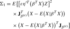
where $\Sigma_{s}=E\{(\varepsilon\eta'^{T}(\beta^{T}X)Z)^{2}e_{s}^{T}\mathbf{J}_{\beta^{(r)}}^{T}(X-E(X|\beta^{T}X))\*(X-E(X|\beta^{T}X))^{T}\mathbf{J}_{\beta^{(r)}}e_{s}\}$.

Proof

(i) By the definition of $\hat{\xi}_{i,s}(\beta_{s})$, we can obtain that

(A.1)

By the central limit theorem with condition (C ₄), it follows

(A.2)

Therefore, to prove Lemma 1(i), we need only to show that $\frac{1}{\sqrt{n}}\sum_{i=1}^{n}\Theta_{il}\stackrel{p}{\longrightarrow }0,\ l=2,3,4,5,6$.

By a Taylor expansion, we can obtain that

(A.3)

and from (A.3) we can derive that

(A.4)

Note that some simple calculation yields

From Lemma 1, and by using the Cauchy-Schwarz inequality and the conditions C ₁, C ₂ and C ₃, we can derive that

(A.5)

By the Markov inequality, we obtain that $A_{3}\stackrel{p}{\longrightarrow}0$, and similarly we can prove $A_{k}\stackrel{p}{\longrightarrow}0$, k=1,2,4. This implies $\frac{1}{\sqrt{n}}\sum_{i=1}^{n}\Theta_{i2}\stackrel{p}{\longrightarrow}0$. Similarly, we have $\frac{1}{\sqrt{n}}\*\sum_{i=1}^{n}\Theta_{i3}\stackrel{p}{\longrightarrow}0$.

Next we consider the proof related to $\frac{1}{\sqrt{n}}\sum_{i=1}^{n}\Theta_{i4}$.

As the expression (A.3), we can obtain that

(A.6)

Thus, by using simple calculation we obtain

(A.7)

By using Lemma 1 and arguments similar to those used in the proof of $\frac{1}{\sqrt{n}}\sum_{i=1}^{n}\Theta_{i2}$, it follows $B_{j}\stackrel{p}{\longrightarrow}0,\ j=1,3$. As to B ₂, we have

(A.8)

By using arguments similar to those for (A.5) and the result (A.4), we can easily show that $B_{2l}\stackrel{p}{\longrightarrow}0,\quad l=1,2,3,4$, which implies that $B_{2}\stackrel{p}{\longrightarrow}0$. Therefore, we conclude $\frac{1}{\sqrt{n}}\sum_{i=1}^{n}\Theta_{i4}\stackrel{p}{\longrightarrow }0$. Similarly, we can also show that $\frac{1}{\sqrt{n}}\sum_{i=1}^{n}\Theta_{i5}\stackrel{p}{\longrightarrow}0$ and $\frac{1}{\sqrt{n}}\sum_{i=1}^{n}\Theta_{i6}\stackrel{p}{\longrightarrow}0$. Hence we complete the proof of Lemma 2(i).

(ii) We use the notations in the proof of the first term. Define $\Theta_{i}^{\star}=\Theta_{i2}+\Theta_{i3}+\Theta_{i4}+\Theta_{i5}+\Theta_{i6}$. Thus

By using the law of large numbers, we can prove that $\Upsilon_{1}\stackrel{p}{\longrightarrow}\Sigma_{s}$. Similarly to Lemma 5 in Zhu and Xue (2006), it can be shown that $\Upsilon_{k}\stackrel{p}{\longrightarrow}0,\quad k=2,3,4$. The proof is completed.

(iii) Notice for any sequence of independent and identically distributed random variables ζ _i , i=1,…,n, with $E(\zeta_{i}^{T}\zeta_{i})<\infty$, we have max_1≤i≤n ∥ζ _i ∥=o _p (n ^1/2). Thus we establish max_1≤i≤n |Θ _i1|=o _p (n ^1/2). Similarly to Lemma 6 in Zhu and Xue (2006), it can be shown that max_1≤i≤n |Θ _ik |=o _p (n ^1/2), k=2,3,4,5,6. The proof is completed.

In addition, together with Lemma 1(ii) and using the arguments similar to Owen (1990), one can prove that |λ|=O _p (n ^−1/2); here we omit the details of the proof. □

Lemma 3

Under the assumptions of Theorem 4, if η(x) is the true value of the parameter, it follows

$$\everymath{\displaystyle} \begin{array}{r@{\quad}l}(\mathrm{i})& \frac{1}{\sqrt{nb}}\sum_{i=1}^{n}\hat{\varphi}_{i} (\eta(x) )\stackrel {d}{\longrightarrow}N(0,\Sigma(x) ),\\\noalign{\vspace{6pt}}(\mathrm{ii})&\frac{1}{nb}\sum_{i=1}^{n}\hat{\varphi}_{i} (\eta(x) )\hat{\varphi }_{i}^{T}(\eta(x) )\stackrel{p}{\longrightarrow}\Sigma(x),\\\noalign{\vspace{6pt}}(\mathrm{iii})&\max_{1\leq i\leq n}\bigl\|\hat{\varphi}_{i} (\eta(x) )\bigr\|=o_{p} ((nb)^{1/2} ),\\\noalign{\vspace{6pt}}& \theta=O_{p} ((nb)^{-1/2} ),\end{array}$$

where Σ(x)=σ ²(x)E(ZZ ^T|β ^T X=x)f(x)∫K ²(t)dt, σ ²(x)=E(ε ²|β ^T X=x).

Proof

By the expression (i) and using the arguments similar to those used in Lemma 2(ii), one can obtain Part (ii). Here we only present the proofs of the expressions (i) and (iii).

From the definition of $\hat{\varphi}_{i}(\eta(x))$ and by using the Taylor expansion, we can write

(A.9)

By using the fact that, for every i

(A.10)

and the result $\hat{\beta}-\beta=O_{p}(n^{-1/2})$ from Theorem 1, by simple calculation we obtain

(A.11)

Further, by the Central Limit Theorem we can establish that

(A.12)

Next we prove $\Delta_{2}\stackrel{p}{\longrightarrow}0$. Noting that

simple calculations give

(A.13)

By using (A.10) and the arguments similar to those used in (i), we can prove that

(A.14)

which, combining with (A.9)–(A.14), leads to (i) of Lemma 3.

As to part (iii), by Lemma 3(i), we can verify that $\frac{1}{nb}\sum_{i=1}^{n}\hat{\varphi}_{i}(\eta(x))=O_{p}((nb)^{-1/2})$. This, combining with Lemma 3(ii), results in the second equation of (iii) by using the same arguments involved in the proof of expression (2.14) in Owen (1990). Next we consider the proof of the expression $\max_{1\leq i\leq n}\|\hat{\varphi}_{i}(\eta(x))\|=o_{p}((nb)^{1/2})$.

Write

It is easy to show that

Here we only need to prove that Ξ _k =o _p ((nb)^1/2), k=1,2,3. Similarly to the proof of the above Lemma 3(i), we can obtain that Ξ _l =o _p ((nb)^1/2), l=1,2,3. Therefore, the proof of Lemma 3 is completed. □

Proof of Theorem 1

By the definition of $\hat{\beta}^{(r)}$, we have

where

By using a method similar to the one applied in Theorem 2 of Wang et al. (2010) and Lemma 1, we can show that

By using the fact that $\sqrt{n}(\hat{\beta}-\beta)=\sqrt{n}\mathbf{J}_{\beta^{(r)}}(\hat{\beta}^{(r)}-\beta^{(r)})(1+o_{p}(1))$ and the Central Limit Theorem, we complete the proof of Theorem 1. □

Proof of Theorem 3

By applying a Taylor series expansion to (11) and invoking Lemma 2, we can show that

(A.15)

By using the expression (12), we have

Further, Lemma 2 results in the following two equations

which, combining with ( A.15 ), leads to

This, together with Lemma 2, completes the proof of Theorem 3. □

Proof of Theorem 4

By applying a Taylor series expansion to (16) and invoking Lemma 3, we can show that

Similar to the proof of Theorem 3, we can complete the proof of Theorem 4; here the details are omitted. □

Proof of Theorem 5

By using the methods applied in Theorem 4, one can complete the proof; here we omit its details. □

References

Cai, Z., Fan, J., Yao, Q.: Functional-coefficient regression models for nonlinear time series. J. Am. Stat. Assoc. 95, 941–956 (2000)
Carroll, R.J., Fan, J., Gijbels, I., Wand, M.P.: Generalized partially linear single-index models. J. Am. Stat. Assoc. 92, 477–489 (1997)
Fan, J., Gijbels, I.: Local Polynomial Modeling and Its Applications. Chapman & Hall, London (1996)
Fan, J.Q., Zhang, W.Y.: Statistical estimation in varying-coefficient models. Ann. Math. Stat. 27, 1491–1518 (1999)
Fan, J.Q., Yao, Q.W., Cai, Z.W.: Adaptive varying-coefficient linear models. J. R. Stat. Assoc. B 65, 57–80 (2003)
Härdle, W., Hall, P., Ichimura, H.: Optimal smoothing in single-index models. Ann. Math. Stat. 21, 157–178 (1993)
Hastie, T.J., Tibshirani, R.: Varying-coefficient models. J. R. Stat. Assoc. B 55, 757–796 (1993)
Ichimura, H.: Semiparametric least squares (SLS) and weighted SLS estimation of singleindex models. J. Econom. 58, 71–120 (1993)
Lu, Z.D., Tjøstheim, D., Yao, Q.W.: Adaptive varying-coefficient linear models for stochastic processes: asymptotic theory. Stat. Sin. 17, 177–197 (2007)
Owen, A.B.: Empirical likelihood ratio confidence intervals for a single function. Biometrika 75, 237–249 (1988)
Owen, A.B.: Empirical likelihood ratio confidence regions. Ann. Math. Stat. 18, 90–120 (1990)
Wang, J.L., Xue, L.G., Zhu, L.X., Chong, Y.S.: Estimation for a partial-linear single-index model. Ann. Math. Stat. 38, 246–274 (2010)
Wu, C.O., Chiang, C.T., Hoover, D.R.: Asymptotic confidence regions for kernel smoothing of a varying-coefficient model with longitudinal data. J. Am. Stat. Assoc. 93, 1388–1402 (1998)
Xia, Y.C., Li, W.K.: On single-index coefficient regression models. J. Am. Stat. Assoc. 94, 1275–1285 (1999a)
Xia, Y.C., Li, W.K.: On the estimation and testing of functional-coefficient linear models. Stat. Sin. 9, 737–757 (1999b)
Xue, L.G., Zhu, L.X.: Empirical likelihood for single-index model. J. Multivar. Anal. 97, 1295–1312 (2006)
Xue, L.G., Zhu, L.X.: Empirical likelihood for a varying coefficient model with longitudinal data. J. Am. Stat. Assoc. 102, 642–654 (2007)
Yu, Y., Ruppert, D.: Penalized spline estimation for partially linear single-index models. J. Am. Stat. Assoc. 97, 1042–1054 (2002)
Zhu, L.X., Xue, L.G.: Empirical likelihood confidence regions in a partially linear single-index model. J. R. Stat. Assoc. B 68, 549–570 (2006)
Acknowledgements
The authors would like to thank Editor and referees for their truly helpful comments and suggestions which led to a much improved presentation.
Author information
Authors and Affiliations
Corresponding author
Additional information
Zhensheng Huang’s research was supported by the National Natural Science Foundation of China (grant 11101114); Riquan Zhang’s research was supported in part by National Natural Science Foundation of China (10871072 and 11171112), Doctoral Fund of Ministry of Education of China (20090076110001).