
Abstract
Recovering the 3D shape of a non-rigid object is a challenging problem. Existing methods make the low-rank assumption and do not scale well with the increased degree of freedom found in complex non-rigid deformations or shape variations. Moreover, in general, the degree of freedom of deformation is assumed to be known in advance, which limits the applicability of non-rigid structure from motion algorithms in a practical situation. In this paper, we propose a method for handling complex shape variations based on the assumption that complex shape variations can be represented probabilistically by a mixture of primitive shape variations. The proposed model is a generative probabilistic model, called a Procrustean normal distribution mixture model, which can model complex shape variations without rank constraints. Experimental results show that the proposed method significantly outperforms existing methods.


Notes
\({\mathbf {Q}}^T {\mathbf {Q}}= {\mathbf {I}}\) but \({\mathbf {Q}}{\mathbf {Q}}^T \ne {\mathbf {I}}\).
In this paper, we use \({\mathbf {0}}\) to denote both matrices and vectors of zeros.
Let \({\mathbf {R}}_i^f\) be a rotation matrix obtained from the factorization method. Then \({\mathbf {R}}_i\) in (32) is a transpose of \({\mathbf {R}}^f\).
The maximum number of shape basis vectors is limited up to \(\lfloor \frac{28}{3}\rfloor \) when the number of landmarks is 28 (Gotardo and Martinez 2011).
Naming convention: \(p \langle n \rangle \_\langle a \rangle \_\langle k \rangle \), where n is the number of persons, a is the action type, and k is the take number.
The maximum number of shape basis vectors is limited up to \(\lfloor \frac{15}{3}\rfloor \) for 15 landmarks (Gotardo and Martinez 2011).
In this table, we denote six sequences as only action types.
The viewpoint of each video sequence is assigned to one of four coarse camera viewpoints, i.e., front, back, left, and right.
We select a more plausible result between the reconstructed 3D shape and its depth inverted version to remove the sign ambiguity. Also, we made two virtual 3D landmarks of a torso, i.e., upper body and lower body, for the purpose of visualization, since the Penn Action dataset does not give torso landmark positions.
Fig. 11 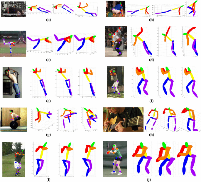
Successful reconstruction results from the Penn Action dataset. Images from the left to right correspond to the 2D input image, 3D reconstruction results of PND, PNDMM, and adaptive PNDMM, respectively. Markers “o” in a 2D input image correspond to the 2D observations and marker colors correspond to body parts according to the reconstruction results

References
Akhter, I., Sheikh, Y., & Khan, S. (2009). In defense of orthonormality constraints for nonrigid structure from motion. In Proceedings of the IEEE Conference on Computer Vision and Pattern Recognition, doi:10.1109/CVPR.2009.5206620.
Akhter, I., Sheikh, Y., Khan, S., & Kanade, T. (2011). Trajectory space: A dual representation for nonrigid structure from motion. IEEE Transactions on Pattern Analysis and Machine Intelligence, 33(7), 1442–1456. doi:10.1109/TPAMI.2010.201.
Bregler, C., Hertzmann, A., & Biermann, H. (2000). Recovering non-rigid 3D shape from image streams. In Proceedings of the IEEE Conference on Computer Vision and Pattern Recognition, doi:10.1109/CVPR.2000.854941.
Celeux, G., Chrétien, S., Forbes, F., & Mkhadri, A. (2001). A component-wise EM algorithm for mixtures. Journal of Computational and Graphical Statistics, 10(4), 697–712.
Cho, J., Lee, M., Choi, C.-H., & Oh, S. (2013). EM-GPA: Generalized Procrustes analysis with hidden variables for 3D shape modeling. Computer Vision and Image Understanding, 117(11), 1549–1559. doi:10.1016/j.cviu.2013.07.009.
Dai, Y., Li, H., & He, M. (2012). A simple prior-free method for non-rigid structure-from-motion factorization. In Proceedings of the IEEE Conference on Computer Vision and Pattern Recognition, doi:10.1109/CVPR.2012.6247905.
Fayad, J., Agapito, L., & Del Bue, A. (2010). Piecewise quadratic reconstruction of non-rigid surfaces from monocular sequences. In Proceedings of the European Conference on Computer Vision, doi:10.1007/978-3-642-15561-1_22.
Figueiredo, M. A. T., & Jain, A. K. (2002). Unsupervised learning of finite mixture models. IEEE Transactions on Pattern Analysis and Machine Intelligence, 24(3), 381–396. doi:10.1109/34.990138.
Forsyth, D.A., & Ponce, J. (2002). Computer vision: A modern approach. Prentice Hall Professional Technical Reference.
Gotardo, P. F., & Martinez, A. M. (2011). Non-rigid structure from motion with complementary rank-3 spaces. In Proceedings of the IEEE Conference on Computer Vision and Pattern Recognition, doi:10.1109/TPAMI.2007.70752.
Lee, M., Cho, J., Choi, C.-H., & Oh, S. (2013). Procrustean normal distribution for non-rigid structure from motion. In Proceedings of the IEEE Conference on Computer Vision and Pattern Recognition, doi:10.1109/TPAMI.2007.70752.
Lee, M., Choi, C.-H., & Oh, S. (2014). A Procrustean Markov process for non-rigid structure recovery. In Proceedings of the IEEE Conference on Computer Vision and Pattern Recognition, doi:10.1109/CVPR.2014.201.
Lin, Z., Chen, M., & Ma, Y. (2010). The augmented lagrange multiplier method for exact recovery of corrupted low-rank matrices. arXiv preprint, arXiv:1009.5055.
Liu, G., Lin, Z., Yan, S., Sun, J., Yu, Y., & Ma, Y. (2013). Robust recovery of subspace structures by low-rank representation. IEEE Transactions on Pattern Analysis and Machine Intelligence, 35(1), 171–184. doi:10.1109/TPAMI.2012.88.
Paladini, M., Del Bue, A., Stosic, M., Dodig, M., Xavier, J., & Agapito, L. (2009). Factorization for non-rigid and articulated structure using metric projections. In Proceedings of the IEEE Conference on Computer Vision and Pattern Recognition, doi:10.1109/CVPR.2009.5206602.
Pizarro, D., & Bartoli, A. (2011). Global optimization for optimal generalized Procrustes analysis. In Proceedings of the IEEE Conference on Computer Vision and Pattern Recognition, doi:10.1109/CVPR.2011.59955677.
Salzmann, M., Urtasun, R., & Fua, P. (2008). Local deformation models for monocular 3D shape recovery. In Proceedings of the IEEE Conference on Computer Vision and Pattern Recognition, doi:10.1109/CVPR.2008.4587499.
Taylor, J., Jepson, A. D., & Kutulakos, K. N. (2010). Non-rigid structure from locally-rigid motion. In Proceedings of the IEEE Conference on Computer Vision and Pattern Recognition, doi:10.1109/CVPR.2010.5540002.
Tomasi, C., & Kanade, T. (1992). Shape and motion from image streams under orthography: A factorization method. International Journal of Computer Vision, 9(2), 137–154. doi:10.1007/BF00129684.
Torresani, L., Hertzmann, A., & Bregler, C. (2008). Nonrigid structure-from-motion: Estimating shape and motion with hierarchical priors. IEEE Transactions on Pattern Analysis and Machine Intelligence, 30(5), 878–892. doi:10.1109/TPAMI.2007.70752.
van der Aa, N., Luo, X., Giezeman, G., Tan, R., & Veltkamp, R. (2011). Utrecht multi-person motion (UMPM) benchmark: A multi-person dataset with synchronized video and motion capture data for evaluation of articulated human motion and interaction. In Proceedings of the Workshop on Human Interaction in Computer Vision, doi:10.1109/ICCVW.2011.6130396.
Varol, A., Salzmann, M., Tola, E., & Fua, P. (2009). Template-free monocular reconstruction of deformable surfaces. In Proceedings of the IEEE International Conference on Computer Vision, doi:10.1109/ICCV.2009.5459403.
Xiao, J., Chai, J., & Kanade, T. (2006). A closed-form solution to non-rigid shape and motion recovery. International Journal of Computer Vision, 67(2), 233–246. doi:10.1007/978-3-540-24673-2_46.
Zelditch, M. L., Swiderski, D. L., & Sheets, H. D. (2012). Geometric morphometrics for biologists: A primer. San Diego: Elsevier/Academic Press.
Zhang, W., Zhu, M., & Derpanis, K. (2013). From actemes to action: A strongly-supervised representation for detailed action understanding. In Proceedings of the IEEE International Conference on Computer Vision, doi:10.1109/ICCV.2013.280.
Zhu, Y., Cox, M., & Lucey, S. (2013). 3D motion reconstruction for real-world camera motion. In Proceedings of the IEEE Conference on Computer Vision and Pattern Recognition, doi:10.1109/CVPR.2011.5995650.
Zhu, Y., Huang, D., Torre, F. D. L., & Lucey, S. (2014). Complex non-rigid motion 3D reconstruction by union of subspaces. In Proceedings of the IEEE Conference on Computer Vision and Pattern Recognition, doi:10.1109/CVPR.2014.200.
Zhu, Y., & Lucey, S. (2015). Convolutional sparse coding for trajectory reconstruction. IEEE Transactions on Pattern Analysis and Machine Intelligence, 37(3), 529–540. doi:10.1109/TPAMI.2013.2295311.
Acknowledgments
This work was supported by Basic Science Research Program through the National Research Foundation of Korea (NRF) funded by the Ministry of Science, ICT & Future Planning (NRF-2013R1A1A2065551).
Author information
Authors and Affiliations
Corresponding author
Additional information
Communicated by Deva Ramanan.
Appendix: Calculation of \(p({\mathbf {X}}_i|{\mathbf {D}}_i, {\varvec{\Phi }}_i)\) in (16)
Appendix: Calculation of \(p({\mathbf {X}}_i|{\mathbf {D}}_i, {\varvec{\Phi }}_i)\) in (16)
This appendix section describes the effect of ignoring the Dirac-delta term in (16).
1.1 Without the Dirac-Delta Term in (16)
We omit subscripts i, k, and ik if no confusion arises. Using Bayes’ rule, the posterior distribution of \({\mathbf {X}}\) can be written as
where \({\mathbf {H}}= s^2 ({\mathbf {I}}\otimes {\mathbf {R}}^T) {\varvec{\Sigma }}^+ ({\mathbf {I}}\otimes {\mathbf {R}}) + \frac{1}{\sigma ^2} {\mathbf {F}}\) and we use \({\mathbf {vec}}(\overline{{\mathbf {X}}})^T {\mathbf {Q}}= 0\), \({\mathbf {vec}}({\mathbf {D}}) = {\mathbf {F}}{\mathbf {vec}}({\mathbf {D}})\), and \({\mathbf {F}}^2 = {\mathbf {F}}\).
We can also write \(p({\mathbf {X}}|{\mathbf {D}}, {\varvec{\Phi }})\) as:
Comparing (35) with (34), we have
Therefore, we can represent \(p({\mathbf {X}}|{\mathbf {D}}, {\varvec{\Phi }})\) as the following Gaussian distribution:
1.2 With the Dirac-Delta Term in (16)
Let \({\mathbf {v}}\) be a random vector drawn from \({\mathcal {N}}({\mathbf {0}}, \Sigma _R)\). Then, \({\mathbf {vec}}({\mathbf {X}})\) can be represented as follows:
By substituting (38) to \({\mathbf {vec}}({\mathbf {X}})\) of (35) in Section 1 and rearranging them with respect to \({\mathbf {v}}\), it can be written as
Since (39) has only a quadric term and a linear term of \({\mathbf {v}}\), and a constant term, it can be represented as
Comparing (39) with (40), we can write
where \(\big ( {\mathbf {vec}}({\mathbf {D}}) - \frac{1}{s} {\mathbf {F}}\left( {\mathbf {I}}\otimes {\mathbf {R}}^T\right) {\mathbf {vec}}(\overline{{\mathbf {X}}}) \big )\) corresponds to non-rigid variations and we can see only non-rigid variations affect \({\widehat{{\mathbf {m}}}}\) since \({\mathbf {Q}}\) is orthogonal to rigid variations by the definition of PND.
\({\mathbf {X}}\) can be consider a linear transformed and translated version of \({\mathbf {v}}\) as shown in (38). By a linear property of a Gaussian distribution, we can also represent \(p({\mathbf {X}}|{\mathbf {D}}, {\varvec{\Phi }})\) as a Gaussian distribution as
where \(({\mathbf {vec}}({\mathbf {D}}) - \frac{1}{s} {\mathbf {F}}\left( {\mathbf {I}}\otimes {\mathbf {R}}^T\right) {\mathbf {vec}}(\overline{{\mathbf {X}}}))\) corresponds to non-rigid variations and \((\frac{1}{s} \left( {\mathbf {I}}\otimes {\mathbf {R}}^T\right) {\mathbf {vec}}(\overline{{\mathbf {X}}}))\) corresponds to rigid ones.
Since \({\mathbf {Q}}\) is a orthogonal to a subspace, \({\mathbf {Q}}_N(\overline{{\mathbf {X}}})\), on rigid motions, it means that we only consider an aligned prior mean shape \(\frac{1}{s}{\mathbf {R}}^T \overline{{\mathbf {X}}}\) and non-rigid variations orthogonal to \(\overline{{\mathbf {X}}}\) and other rigid variations are removed by \({\mathbf {Q}}\). However, we empirically found ignoring the Dirac-delta term makes the distribution \(p({\mathbf {X}}|{\mathbf {D}}, {\varvec{\Phi }})\) close to the observation \({\mathbf {D}}\) and gives better reconstruction results, since s and \({\mathbf {R}}\) have inexact values in the early stage of the iteration process.
Rights and permissions
About this article

Cite this article
Cho, J., Lee, M. & Oh, S. Complex Non-rigid 3D Shape Recovery Using a Procrustean Normal Distribution Mixture Model. Int J Comput Vis 117, 226–246 (2016). https://doi.org/10.1007/s11263-015-0860-7
Received:
Accepted:
Published:
Issue Date:
DOI: https://doi.org/10.1007/s11263-015-0860-7