
Abstract
This work focuses on elucidating issues related to an increasingly common technique of multi-model ensemble (MME) forecasting. The MME approach is aimed at improving the statistical accuracy of imperfect time-dependent predictions by combining information from a collection of reduced-order dynamical models. Despite some operational evidence in support of the MME strategy for mitigating the prediction error, the mathematical framework justifying this approach has been lacking. Here, this problem is considered within a probabilistic/stochastic framework which exploits tools from information theory to derive a set of criteria for improving probabilistic MME predictions relative to single-model predictions. The emphasis is on a systematic understanding of the benefits and limitations associated with the MME approach, on uncertainty quantification, and on the development of practical design principles for constructing an MME with improved predictive performance. The conditions for prediction improvement via the MME approach stem from the convexity of the relative entropy which is used here as a measure of the lack of information in the imperfect models relative to the resolved characteristics of the truth dynamics. It is also shown how practical guidelines for MME prediction improvement can be implemented in the context of forced response predictions from equilibrium with the help of the linear response theory utilizing the fluctuation–dissipation formulas at the unperturbed equilibrium. The general theoretical results are illustrated using exactly solvable stochastic non-Gaussian test models.


References
Abramov, R.V., Majda, A.J.: Quantifying uncertainty for non-Gaussian ensembles in complex systems. SIAM J. Sci. Comput. 26, 411–447 (2004)
Abramov, R.V., Majda, A.J.: Blended response algorithms for linear fluctuation-dissipation for complex nonlinear dynamical systems. Nonlinearity 20(12), 2793–2821 (2007)
Anderson, J.L.: An adaptive covariance inflation error correction algorithm for ensemble filters. Tellus 59A, 210–224 (2007)
Arnold, L.: Random Dynamical Systems. Springer, New York (1998)
Branicki, M., Majda, A.J.: Dynamic stochastic superresolution of sparsely observed dynamical systems. J. Comput. Phys. 241, 333–363 (2012a)
Branicki, M., Majda, A.J.: Fundamental limitations of polynomial chaos for uncertainty quantification in systems with intermittent instabilities. Commun. Math. Sci. 11(1) (2012b)
Branicki, M., Majda, A.J.: Quantifying uncertainty for statistical predicions with model errors in non-Gaussian models with intermittency. Nonlinearity 25, 2543–2578 (2012c)
Branicki, M., Majda, A.J.: Quantifying Bayesian filter performance for turbulent dynamical systems through information theory. Commun. Math. Sci. 12(5), 901–978 (2014)
Branicki, M., Gershgorin, B., Majda, A.J.: Filtering skill for turbulent signals for a suite of nonlinear and linear Kalman filters. J. Comput. Phys. 231, 1462–1498 (2012)
Chatterjee, A., Vlachos, D.: An overview of spatial microscopic and accelerated kinetic Monte Carlo methods. J. Comput. Aided Mater. 14, 253–308 (2007)
Chen, N., Majda, A.J., Giannakis, D.: Predicting the cloud patterns of the Madden–Julian oscillation through a low-order nonlinear stochastic model. Geophys. Res. Lett. 41(15), 5612–5619 (2014a)
Chen, N., Majda, A.J., Tong, X.T.: Information barriers for noisy Lagrangian tracers in filtering random incompressible flows. Nonlinearity 27(9), 2133 (2014b)
Cover, T.A., Thomas, J.A.: Elements of Information Theory. Wiley-Interscience, Hoboken (2006)
Das, P., Moll, M., Stamati, H., Kavraki, L.E., Clementi, C.: Low-dimensional, free energy landscapes of protein-folding reactions by nonlinear dimensionality reduction. Proc. Natl. Acad. Sci. 103, 9885–9890 (2006)
Doblas-Reyes, F.J., Hagedorn, R., Palmer, T.N.: The rationale behind the success of multi-model ensembles in seasonal forecasting. Part II: calibration and combination. Tellus Ser. A 57, 234–252 (2005)
Emanuel, K.A., Wyngaard, J.C., McWilliams, J.C., Randall, D.A., Yung, Y.L.: Improving the Scientific Foundation for Atmosphere-Land Ocean Simulations. National Academy Press, Washington, DC (2005)
Epstein, E.S.: Stochastic dynamic predictions. Tellus 21, 739–759 (1969)
Gershgorin, B., Majda, A.J.: Quantifying uncertainty for climate change and long range forecasting scenarios with model errors. Part I: Gaussian models. J. Clim. 25, 4523–4548 (2012)
Gershgorin, B., Harlim, J., Majda, A.J.: Improving filtering and prediction of spatially extended turbulent systems with model errors through stochastic parameter estimation. J. Comput. Phys. 229, 32–57 (2010a)
Gershgorin, B., Harlim, J., Majda, A.J.: Test models for improving filtering with model errors through stochastic parameter estimation. J. Comput. Phys. 229, 1–31 (2010b)
Giannakis, D., Majda, A.J.: Quantifying the predictive skill in long-range forecasting. Part I: coarse-grained predictions in a simple ocean model. J. Clim. 25, 1793–1813 (2012a)
Giannakis, D., Majda, A.J.: Quantifying the predictive skill in long-range forecasting. Part II: model error in coarse-grained Markov models with application to ocean-circulation regimes. J. Clim. 25, 1814–1826 (2012b)
Giannakis, D., Majda, A.J., Horenko, I.: Information theory, model error, and predictive skill of stochastic models for complex nonlinear systems. Phys. D 241(20), 1735–1752 (2012)
Gibbs, A.L., Su, F.E.: On choosing and bounding probability metrics. Int. Stat. Rev. 70(3), 419–435 (2002)
Gritsun, A., Branstator, G., Majda, A.J.: Climate response of linear and quadratic functionals using the fluctuation–dissipation theorem. J. Atmos. Sci. 65, 2824–2841 (2008)
Grooms, I., Majda, A.J.: Efficient stochastic superparameterization for geophysical turbulence. Proc. Natl. Acad. Sci. 110(12), 4464–4469 (2013)
Grooms, I., Majda, A.J.: Stochastic superparameterization in quasigeostrophic turbulence. J. Comput. Phys. 271, 78–98 (2014)
Grooms, I., Lee, Y., Majda, A.J.: Ensemble Kalman filters for dynamical systems with unresolved turbulence. J. Comput. Phys. 273, 435–452 (2014)
Grooms, I., Majda, A.J., Smith, K.S.: Stochastic superparameterization in a quasigeostrophic model of the antarctic circumpolar current. Ocean Model 85, 1–15 (2015)
Hagedorn, R., Doblas-Reyes, F.J., Palmer, T.N.: The rationale behind the success of multi-model ensembles in seasonal forecasting. Part I: basic concept. Tellus 57A, 219–233 (2005)
Hairer, M., Majda, A.J.: A simple framework to justify linear response theory. Nonlinearity 12, 909–922 (2010)
Harlim, J., Majda, A.J.: Filtering turbulent sparsely observed geophysical flows. Mon. Weather. Rev. 138(4), 1050–1083 (2010)
Houtekamer, P., Mitchell, H.: A sequential ensemble Kalman filter for atmospheric data assimilation. Mon. Weather Rev. 129, 123–137 (2001)
Hummer, G., Kevrekidis, I.G.: Coarse molecular dynamics of a peptide fragment: free energy, kinetics and long-time dynamics computations. J. Chem. Phys. 118, 10762–10773 (2003)
Katsoulakis, M.A., Majda, A.J., Vlachos, D.: Coarse-grained stochastic processes for microscopic lattice systems. Proc. Natl. Acad. Sci. 100, 782–787 (2003)
Kim, H.-M., Webster, P.J., Curry, J.A.: Evaluation of short-term climate change prediction in multi-model CMIP5 decadal hindcasts. Geophys. Res. Lett. 39, L10701 (2012)
Kleeman, R.: Measuring dynamical prediction utility using relative entropy. J. Atmos. Sci. 59(13), 2057–2072 (2002)
Kleeman, R., Majda, A.J., Timofeyev, I.I.: Quantifying predictability in a model with statistical features of the atmosphere. Proc. Natl. Acad. Sci. 99, 15291–15296 (2002)
Kullback, S., Leibler, R.: On information and sufficiency. Ann. Math. Stat. 22, 79–86 (1951)
Leith, C.E.: Climate response and fluctuation dissipation. J. Atmos. Sci. 32, 2022–2025 (1975)
Lorenz, E.N.: A study of predictability of a 28-variable atmospheric model. Tellus 17, 321–333 (1968)
Lorenz, E.N.: The predictability of a flow which possesses many scales of motion. Tellus 21, 289–307 (1969)
Majda, A.J.: Real world turbulence and modern applied mathematics. In: Arnold, V.I. (ed.) Mathematics: Frontiers and Perspectives, pp. 137–151. American Mathematical Society, Providence, RI (2000)
Majda, A.J.: Challenges in climate science and contemporary applied mathematics. Commun. Pure Appl. Math. 65(7), 920–948 (2012)
Majda, A.J., Wang, X.: Nonlinear Dynamics and Statistical Theories for Basic Geophysical Flows. Cambridge University Press, Cambridge (2006)
Majda, A.J., Gershgorin, B.: Quantifying uncertainty in climate change science through empirical information theory. Proc. Natl. Acad. Sci. 107(34), 14958–14963 (2010)
Majda, A.J., Wang, X.: Linear response theory for statistical ensembles in complex systems with time-periodic forcing. Commun. Math. Sci. 8(1), 145–172 (2010)
Majda, A.J., Gershgorin, B.: Improving model fidelity and sensitivity for complex systems through empirical information theory. Proc. Natl. Acad. Sci. 108(31), 10044–10049 (2011a)
Majda, A.J., Gershgorin, B.: Link between statistical equilibrium fidelity and forecasting skill for complex systems with model error. Proc. Natl. Acad. Sci. 108(31), 12599–12604 (2011b)
Majda, A.J., Branicki, M.: Lessons in uncertainty quantification for turbulent dynamical systems. Discrete Contin Dyn. Syst. 32(9), 3133–3231 (2012)
Majda, A.J., Harlim, J.: Filtering Complex Turbulent Systems. Cambridge University Press, Cambridge, MA (2012)
Majda, A.J., Yuan, Y.: Fundamental limitations of ad hoc linear and quadratic multi-level regression models for physical systems. Discrete Cont. Dyn. Syst. 4, 1333–1363 (2012)
Majda, A.J., Grooms, I.: New perspectives on superparameterization for geophysical turbulence. J. Comput. Phys 271, 60–77 (2014)
Majda, A.J., Lee, Y.: Conceptual dynamical models for turbulence. Proc. Natl. Acad. Sci. 111, 6548–6553 (2014)
Majda, A.J., Kleeman, R., Cai, D.: A mathematical framework for predictability through relative entropy. Methods Appl. Anal. 9(3), 425–444 (2002)
Majda, A.J., Timofeyev, I.I., Vanden Eijnden, E.: Systematic strategies for stochastic mode reduction in climate. J. Atmos. Sci. 60, 1705 (2003)
Majda, A.J., Abramov, R.V., Grote, M.J.: Information Theory and Stochastics for Multiscale Nonlinear Systems, Volume 25 of CRM Monograph Series. Americal Mathematical Society, Providence, RI Providence (2005)
Majda, A.J., Abramov, R.V., Gershgorin, B.: High skill in low frequency climate response through fluctuation dissipation theorems despite structural instability. Proc. Natl. Acad. Sci. 107(2), 581–586 (2010a)
Majda, A.J., Gershgorin, B., Yuan, Y.: Low-frequency climate response and fluctuation-dissipation theorems: theory and practice. J. Atmos. Sci. 67, 1186 (2010b)
Majda, A.J., Harlim, J., Gershgorin, B.: Mathematical strategies for filtering turbulent dynamical systems. Discrete Contin. Dyn. Syst. 27, 441–486 (2010c)
Majda, A.J., Qi, D., Sapsis, T.P.: Blended particle filters for large-dimensional chaotic dynamical systems. Proc. Natl. Acad. Sci. 111(21), 7511–7516 (2014)
Mead, L.R., Papanicolaou, N.: Maximum entropy in the problem of moments. J. Math. Phys. 25(8), 2404–2417 (1984)
Neelin, J.D., Munnich, M., Su, H., Meyerson, J.E., Holloway, C.E.: Tropical drying trends in global warming models and observations. Proc. Natl. Acad. Sci. 103, 6110–6115 (2006)
Noé, F., Schutte, C., Vanden-Eijnden, E., Reich, L., Weikl, T.R.: Constructing the equilibrium ensemble of folding pathways from short off-equilibrium simulations. Proc. Natl. Acad. Sci. 106(45), 19011–19016 (2009)
Øksendal, B.K.: Stochastic Differential Equations: An Introduction with Applications. Springer, Berlin (2010)
Palmer, T.N.: A nonlinear dynamical perspective on model error: a proposal for nonlocal stochastic dynamic parameterizations in weather and climate prediction models. Q. J. R. Meteorol. Soc. 127, 279–303 (2001)
Palmer, T.N., Shutts, G.J., Hagedorn, R., Doblas-Reyes, F.J., Jung, T., Leutbecher, M.: Representing model uncertainty in weather and climate prediction. Ann. Rev. Earth Planet. Sci. 33, 163–193 (2005)
Randall, D.A.: Climate models and their evaluation. In Solomon, S. (eds) Climate Change 2007: The Physical Science Basis, Contribution of Working Group I to the Fourth Assessment Report of the Intergovernmental Panel on Climate change, pp. 589–662. Cambridge University Press, Cambridge, MA (2007)
Rangan, A., Tao, L., Kovacic, G., Cai, D.: Multiscale modeling of the primary visual cortex. IEEE Eng. Med. Biol. Mag. 28(3), 19–24 (2009)
Sapsis, T., Majda, A.J.: A statistically accurate modified quasilinear Gaussian closure for uncertainty quantification in turbulent dynamical systems. Phys. D 252, 34–45 (2013a)
Sapsis, T., Majda, A.J.: Blended reduced subspace algorithms for uncertainty quantification of quadratic systems with a stable mean state. Phys. D 258, 61–76 (2013b)
Sapsis, T., Majda, A.J.: Blending modified Gaussian closure and non-Gaussian reduced subspace methods for turbulent dynamical systems. J. Nonlinear Sci. 23, 1039–1071 (2013c)
Sapsis, T., Majda, A.J.: Statistically accurate low-order models for uncertainty quantification in turbulent dynamical systems. Proc. Natl. Acad. Sci. 110(34), 13705–13710 (2013d)
Slawinska, J., Pauluis, O., Majda, A.J., Grabowski, W.W.: Multi-scale interactions in an idealized Walker circulation: simulations with sparse space-time superparameterization. Mon. Weather Rev. 143, 563–580 (2015)
Sriraman, S., Kevrekidis, I.G., Hummer, G.: Coarse master equation from Bayesian analysis of replica molecular dynamics. J. Phys. Chem. B 109, 6479–6484 (2005)
Stephenson, D.B., Coelho, C.A.S., Doblas-Reyes, F.J., Balmaseda, M.: Forecast assimilation: a unified framework for the combination of multi-model weather and climate predictions. Tellus A 57, 253–264 (2005)
Thual, S., Majda, A.J., Stechmann, S.N.: A stochastic skeleton model for the MJO. J. Atmos. Sci. 71, 697–715 (2014)
van der Linden, P., Mitchell, J.F.B., (eds). Ensembles: Climate Change and Its Impacts: Summary of Research and Results From the Ensembles Project. Met Office Hadley Centre, Fitzroy Road, Exeter EX1 3PB, UK (2009)
van Oldenborgh, G.J., Doblas-Reyes, F.J., Wouters, B., Hazeleger, W.: Decadal prediction skill in a multi-model ensemble. Clim. Dyn. 38, 1263–1280 (2012)
Weigel, A.P., Liniger, M.A., Appenzeller, C.: Can multi-model combination really enhance the prediction skill of probabilistic ensemble forecasts? Q. J. R. Meteorol. Soc. 134, 241–260 (2008)
Weisheimer, A., Doblas-Reyes, F.J., Palmer, T.N., Alessandri, A., Arribas, A., Déqué, M., Keenlyside, N., MacVean, M., Navarra, A., Rogel, P.: ENSEMBLES: a new multi-model ensemble for seasonal-to-annual predictions—skill and progress beyond DEMETER in forecasting tropical Pacific SSTs. Geophys. Res. Lett. 36, L21711 (2009)
Acknowledgments
M.B. was supported as a postdoctoral fellow on the ONR DRI Grant of A.J.M: N0014-10-1-0554. The research of A.J.M. is partially supported by National Science Foundation CMG Grant DMS-1025468 and the Office of Naval Research Grants ONR DRI N0014-10-1-0554, N00014-11-1-0306, and the MURI award ONR-MURI N00014-12-1-0912.
Author information
Authors and Affiliations
Corresponding author
Additional information
Communicated by Paul Newton.
Appendices
Appendix 1: Some Simple Proofs of General Results from Sect. 3
Here, we complement the discussion of Sect. 3 by providing simple derivations and proofs of the facts established in that section.
Information Criterion II in (12) Derivation of this criterion relies on the convexity properties (10) of the relative entropy (e.g., Cover and Thomas 2006), which leads to the following upper bound on the lack of information in the MME mixture density \(\pi ^{\textsc {mme}}_t\) (1) relative to the least-biased estimate of the marginal truth density \(\pi _t\)
where \(\alpha _i\geqslant 0\) and \(\sum _i\alpha _i = 1\) so that
where we used the fact that \({\mathcal {P}}\geqslant 0\). Clearly, the information criterion in (7) is always satisfied when the right-hand side in (55) satisfies

which, after rearranging terms, gives the sufficient condition in (12) with \(\varDelta =0\), i.e.,
This sufficient condition is too restrictive when \({\textsc {m}}_{\diamond }\) coincides with the best imperfect model \({\textsc {m}}^*_{{\mathcal {I}},{\textsc {l}}}\) in (8) since there is no non-trivial MME satisfying (56). Based on the basic convexity properties of the relative entropy illustrated in Fig. 2 and Fact 1, it is clear that unless \({\mathcal {P}}_{\mathcal {I}}(\pi ^{\textsc {l}},\pi ^{{\textsc {m}}^*_{{\mathcal {I}},{\textsc {l}}}})=0\), an MME with a smaller error does exist and the condition (57) needs to be relaxed in order to be applicable in such cases. The uncertainty parameter \(\varDelta \) in
allows for including models in the ensemble with error \({\mathcal {P}}_{\mathcal {I}}(\pi ^{{\textsc {l}}},\pi ^{{\textsc {m}}^*_{{\mathcal {I}},{\textsc {l}}}})\leqslant {\mathcal {P}}_{\mathcal {I}}(\pi ^{{\textsc {l}}},\pi ^{\textsc {m}})<{\mathcal {P}}_{\mathcal {I}}(\pi ^{{\textsc {l}}}, \pi ^{{\textsc {m}}^*_{{\mathcal {I}},{\textsc {l}}}})+\varDelta \) so that the MME prediction error is \(0\leqslant {\mathcal {P}}_{\mathcal {I}}(\pi ^{\textsc {l}},\pi ^{{\textsc {mme}}}) \leqslant {\mathcal {P}}_{\mathcal {I}}(\pi ^{\textsc {l}},\pi ^{{\textsc {m}}_{\diamond }})+\varDelta \), as illustrated in Fig. 2c.
Proof of Fact 3
The proof is straightforward and follows by a direct calculation consisting of two steps:
-
(1)
We start by rewriting the condition (12) in terms of the least-biased densities defined in (14) which leads to
$$\begin{aligned}&{\mathcal {P}}(\pi ^{{\textsc {l}}_1}_t,\pi ^{{\textsc {m}}_{\diamond },{\textsc {l}}_2}_t)+\varDelta > \sum _{i\ne {\diamond }}\beta _i\,{\mathcal {P}}(\pi ^{{\textsc {l}}_1}_t,\pi ^{{\textsc {m}}_i,{\textsc {l}}_2}_t)\nonumber \\&\quad +\,\sum _{i\ne {\diamond }}\beta _i\,{\mathbb {E}}^{\pi ^{{\textsc {l}}_1}} \Big [\log \frac{\pi ^{{\textsc {m}}_i,{\textsc {l}}_2}}{\pi ^{{\textsc {m}}_i}}-\log \frac{\pi ^{{\textsc {m}}_{\diamond },{\textsc {l}}_2}}{\pi ^{{\textsc {m}}_{\diamond }}} \Big ]; \end{aligned}$$(59)note that this last term vanishes identically when \(\pi ^{{\textsc {m}}_i,{\textsc {l}}_2}=\pi ^{{\textsc {m}}_i}\) and the MME contains only least-biased models.
-
(2)
Next, we notice that the relative entropy between two least-biased densities \(\pi ^{{\textsc {l}}_1}_t\) and \(\pi ^{{\textsc {m}},{\textsc {l}}_2}_t\) is given by
$$\begin{aligned} {\mathcal {P}}(\pi ^{{\textsc {l}}_1}_t,\pi ^{{\textsc {m}},{\textsc {l}}_2}_t)&=\log C^{\textsc {m}}_t+{\pmb {\theta }}^{{\textsc {m}}}_t\cdot \bar{\pmb {E}}_t -\big (\log C_t + {\pmb {\theta }}_t\cdot \bar{\pmb {E}}_t\,\big )\nonumber \\&=\log \frac{\;\;C^{\textsc {m}}_t}{C_t}+ ({\pmb {\theta }}^{{\textsc {m}}}_t\!{-}\,\,{\pmb {\theta }}_t)\cdot \bar{\pmb {E}}_t, \end{aligned}$$(60)where \({\overline{\pmb {E}}}_t\) is the vector of expectations of the functionals \(E_i\) defined in (15) with respect to the truth marginal density \(\pi _t\), and the Lagrange multipliers in (14), \({\pmb {\theta }}_t = {\pmb {\theta }}\big ({\overline{\pmb {E}}}_t\big ),\,{\pmb {\theta }}^{{\textsc {m}}}_t = {\pmb {\theta }}^{{\textsc {m}}}\big ({\overline{\pmb {E}}}^{\textsc {m}}_t\big )\), are defined as
$$\begin{aligned} {\pmb {\theta }_t} = (\theta _1(t),\dots ,\theta _{{\textsc {l}}_1}(t))^\text {T}, \quad \,\, {\pmb {\theta }}^{{\textsc {m}}}_t = (\theta _1^{\textsc {m}}(t),\dots ,\theta ^{\textsc {m}}_{{\textsc {l}}_2}(t),0,\dots ,0_{{\textsc {l}}_1})^\text {T}, \quad \,\, {\textsc {l}}_1\geqslant {\textsc {l}}_2, \end{aligned}$$while the normalization constants in the least-biased densities are \(C_t = C\big ({\overline{\pmb {E}}}_t\big ),\,C^{\textsc {m}}_t =C^{\textsc {m}}\big ({\overline{\pmb {E}}}^{\textsc {m}}_t\big )\).
The condition in (16) is obtained by combining (59) with (60).
Proof of Fact 4
The condition in (21) for improvement in the prediction skill via MME in the context of initial value problem can be obtained as follows: Consider the representation of the true expected values \({\overline{\pmb {E}}}_t\) of the functionals \(E_i(\pmb {u})\) with respect to the truth marginal density \(\pi _t(\pmb {u})\) in the form
these are smooth at \(\delta =0\) when the decomposition \(\pi _t=\pi _0+\delta {\tilde{\pi }}_t\) is smooth at \(\delta =0\) which holds under minimal hypothesis described in Hairer and Majda (2010) so that
The lack of information in (12) between the least-biased approximation of the truth \(\pi ^{{\textsc {l}}_1}_t\) and the imperfect model density \(\pi ^{{\textsc {m}}_i}_t\) can be written as
similarly to the result leading to (59). The lack of information in the perturbed least-biased density, \(\pi ^{{\textsc {m}}_i,{\textsc {l}}_2}_t \), of the imperfect model relative to the least-biased perturbation of the truth, \(\pi ^{{\textsc {l}}_1}_t\), can be expressed through (65)–(68) in the following form
Substituting (64) into (16) leads to the desired condition (21). \(\square \)
Proof of Fact 5
The condition in (25) for improvement in the prediction skill via MME obtained by perturbing single-model predictions can be obtained as follows: Consider the condition (16) in the case when the ensemble members \({\textsc {m}}_i\in {\mathcal {M}}\) are obtained from the single model \({\textsc {m}}_{\diamond }\in {\mathcal {M}}\) through perturbing some parameters of the single model; we assume that the statistics of the model depend smoothly on these parameters and that the perturbations are non-singular (which required minimal assumptions Hairer and Majda 2010 of hypoelliptic noise in the truth dynamics) so that the evolution of the statistical moments \({\overline{\pmb {E}}}_t^{{\textsc {m}}_i}\) and their functions in the least-biased densities (60) of the ensemble members can be written, for \(\epsilon \ll 1\), as
where
The lack of information in the perturbed least-biased density, \(\pi ^{{\textsc {m}}_i,{\textsc {l}}_2}_t \), of the imperfect model relative to the least-biased perturbation of the truth, \(\pi ^{{\textsc {l}}_1}_t\), can be expressed through (65)–(68) in the following form
which is obtained by combining (65)–(67). Substituting (69) into the general condition (16) leads to the desired condition (25). \(\square \)
Proof of Fact 6
The proof of the condition (31) is simple but tedious and follows from the short-time asymptotic expansion of the relative entropy between the Gaussian truth and the Gaussian models. Consider the state vector \(\pmb {u}\in {\mathbb {R}}^K\) for resolved dynamics and assume that short times the statistics of the Gaussian truth density \(\pi _t^{{\textsc {g}}}={\mathcal {N}}(\pmb {\mu }_t,R_t)\) and of the Gaussian model density \(\pi ^{{\textsc {m}}_i}_t={\mathcal {N}}(\pmb {\mu }_t^{{\textsc {m}}_i},R_t^{{\textsc {m}}_i})\) are
and
Then, the relative entropy between the Gaussian truth density \(\pi _t^{{\textsc {g}}}\) and a Gaussian model density \(\pi ^{{\textsc {m}}_i}_t\)
with \(\varDelta \pmb {\mu }_t^i:=\pmb {\mu }_t-\pmb {\mu }_t^{{\textsc {m}}_i}\) can be expressed as
which is valid at times short enough so that the changes in moments \(\delta {\tilde{\pmb {\mu }}}, \delta {\tilde{R}},\,\delta {\tilde{\pmb {\mu }}}^{{\textsc {m}}_i}, \delta {\tilde{R}}^{{\textsc {m}}_i}\) are small; the respective coefficients in (73) are given by
For correct initial conditions, \(\pmb {\mu }^{{\textsc {m}}_i}_0=\pmb {\mu }_0,\,R_0^{{\textsc {m}}_i}=R_0\), the above formulas simplify to
with the remaining coefficients identically zero. Substituting the relative entropy between \({\mathcal {P}}(\pi _t^{\textsc {g}},\pi _t^{{\textsc {m}}_i})\) in the form (73) with the coefficients (74)–(75) into the general necessary condition (12) for improving the prediction via MME yields the condition (31). \(\square \)
Proof of Fact 7
We assume that the perturbations of the equilibrium truth and model densities are smooth in response to the forcing perturbations so that the perturbed densities \(\pi ^\delta _t = \pi _\mathrm{eq}+\delta {\tilde{\pi }}_t\) are differentiable at \(\delta =0\); this holds under relatively mild assumptions hypoelliptic noise as shown in (Hairer and Majda 2010). Thus, based on the linear response theory combined with the fluctuation–dissipation formulas (e.g., Majda et al. 2005), the density perturbations remain small for sufficiently small external perturbations which also implies that the moment perturbations remain small for all time. Derivation of the condition (78) relies on the smallness of the moment perturbations which allows for an asymptotic expansion of the relative entropy as in (73) but with \(\pmb {\mu }_0=\pmb {\mu }_\mathrm{eq}=\pmb {\mu }^{{\textsc {m}}_i}_\mathrm{eq},\,R_0=R_\mathrm{eq}=R^{{\textsc {m}}_i}_\mathrm{eq}\) which leads to expansion coefficients in (73)
with the remaining coefficients identically zero. The general condition for improvement in forced response prediction via MME in the Gaussian framework is
where

which is very similar to the condition in FACT 6 except that there is no short-time constraint due to the fact that the moment perturbations remain small in time under the above assumptions. Finally, the simplified result (32) in Fact 7 of Sect. 3.2 is obtained by taking into account that the response is due to the forcing perturbations in linear Gaussian systems (26) so that \({\tilde{R}}^{{\textsc {m}}_i}_t=0\) so that \(X^R=Y^{R,R}=0\) in (76), (77) and only \(D_{\pmb {\beta },{\mathcal {I}}}\), which is independent of the truth response in the covariance, remains in (78).
\(\square \)
Appendix 2: Further Details of Associated with the Sufficient Conditions for Imperfect Prediction Improvement Via MME
In Sect. 3.1.1, we discussed the condition (12) for improving imperfect predictions via MME in the least-biased density representation (16). Here, we discuss the same condition in terms of general perturbations of probability densities which provides additional insight into the essential features of MME with improved prediction skill. In particular, we show that it is difficult to improve the short-term predictive skill via MME containing models with incorrect statistical initial conditions.
The formulation presented below relies on relatively weak assumptions that the truth and model densities can be written as
The above decomposition is always possible for the non-singular initial value problem; in the case of the forced response prediction from equilibrium (i.e., when \(\pi _{0}^{\textsc {l}}=\pi _\mathrm{eq}^{\textsc {l}},\,\pi _{0}^{\textsc {m}}=\pi _\mathrm{eq}^{\textsc {m}}\)), such a decomposition exists for \(\delta \ll 1\) under the minimal assumptions of hypoelliptic noise (Hairer and Majda 2010). The possibility of estimating the evolution of statistical moments of the truth density \(\pi _t\) in the case of predicting the forced response within the framework of linear response theory combined with the fluctuation–dissipation approach makes this framework particularly important in this case (see Majda et al. 2005, 2010b, a; Abramov and Majda 2007; Gritsun et al. 2008; Majda and Gershgorin 2010, 2011a, b)
Fact
Assume the decomposition (79) of the truth and model densities exists as discussed above. Then, the condition (12) for prediction improvement through MME has the following form
where

with the weights \(\beta _i\) defined in (12). The following particular cases of the condition (80) for improving the predictions via the MME approach are worth noting in this general representation:
-
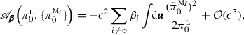
Initial (statistical) conditions in all models of MME are consistent with the least-biased estimate of the truth; i.e., \(\pi ^{{\textsc {m}}_i}_{0}=\pi _{0}^{\textsc {l}}\). In such a case, we have \({\fancyscript{A}}_{\pmb {\beta }}=0,\,{\fancyscript{B}}_{\pmb {\beta },{\mathcal {I}}}=0\) and the condition (80) for improvement in prediction via MME simplifies to
 (81)
(81)In the case of forced response predictions, perturbation of the truth density \({\tilde{\pi }}_t^{\textsc {l}}\) can be estimated from the statistics on the unperturbed equilibrium through the linear response theory and fluctuation–dissipation formulas exploiting only the unperturbed equilibrium information (Majda et al. 2005, 2010b, a; Abramov and Majda 2007; Gritsun et al. 2008; Majda and Gershgorin 2010, 2011a, b).
-
Initial model densities in MME perturbed relative to the least-biased estimate of the truth; i.e., \(\pi ^{{\textsc {m}}_i}_{0}=\pi _{0}^{\textsc {l}}+\epsilon \,{\tilde{\pi }}^{{\textsc {m}}_i}_{0},\,\pi ^{{\textsc {m}}_{\diamond }}_{0}=\pi _{0}^{\textsc {l}}\). In such a case, all terms in (80) are non-trivial but they can be written as
 (82)
(82)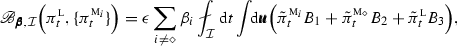 (83)
(83)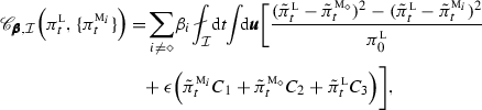 (84)
(84)where \(\{B_m\},\{C_m\},\,m=1,2,3\) are functions of \({\tilde{\pi }}^{{\textsc {m}}_i}_0,{\tilde{\pi }}^{{\textsc {m}}_{\diamond }}_0, {\tilde{\pi }}^{\textsc {l}}_0\) and \(\epsilon \). Note that unless \(\epsilon =0\) (so that \(\pi ^{{\textsc {m}}_i}_{0}=\pi _{0}^{\textsc {l}}\)), it is difficult to improve the prediction skill at short times within the MME framework since at \(t=0\), we have \({\fancyscript{B}}_{\pmb {\beta },{\mathcal {I}}}={\fancyscript{C}}_{\pmb {\beta },{\mathcal {I}}}=0\) and \({\fancyscript{A}}_{\pmb {\beta }}<0\) in (80).


Rights and permissions
About this article

Cite this article
Branicki, M., Majda, A.J. An Information-Theoretic Framework for Improving Imperfect Dynamical Predictions Via Multi-Model Ensemble Forecasts. J Nonlinear Sci 25, 489–538 (2015). https://doi.org/10.1007/s00332-015-9233-1
Received:
Accepted:
Published:
Issue Date:
DOI: https://doi.org/10.1007/s00332-015-9233-1