Iterative scheme-inspired network for impulse noise removal

Abstract

This paper presents a supervised data-driven algorithm for impulse noise removal via iterative scheme-inspired network (IIN). IIN is defined over a data flow graph, which is derived from the iterative procedures in Alternating Direction Method of Multipliers (ADMM) algorithm for optimizing the L1-guided variational model. In the training phase, the L1-minimization is reformulated into an augmented Lagrangian scheme through adding a new auxiliary variable. In the testing phase, it has computational overhead similar to ADMM but uses optimized parameters learned from the training data for restoration task. Experimental results demonstrate that the newly proposed method can obtain very significantly superior performance than current state-of-the-art variational and dictionary learning-based approaches for salt-and-pepper noise removal.

Appendix

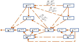
The detailed training procedures of IIN are as follows:

• 1. Multiplier update layer (${\mathbf{M}}^{{\left( {\mathbf{n}} \right)}}$):

This layer has three sets of inputs: $\left\{ {\beta_{l}^{(n - 1)} } \right\},\left\{ {c_{l}^{(n)} } \right\}$ and {z⁽ⁿ⁾_l}. Its output $\left\{ {\beta_{l}^{(n)} } \right\}$ is the input to compute $\left\{ {\beta_{l}^{(n + 1)} } \right\},\left\{ {z_{l}^{(n + 1)} } \right\}$ and $\left\{ {x_{l}^{(n + 1)} } \right\}$. The parameters in this layer are $\left\{ {\eta_{l}^{(n)} } \right\},\;l = \left[ {1,2, \ldots ,L} \right]$. The gradients of loss w.r.t. the parameters can be computed as:

$$\frac{\partial E}{{\partial \eta_{l}^{\left( n \right)} }} = \frac{\partial E}{{\partial \beta_{l}^{\left( n \right)} }}\frac{{\partial \beta_{l}^{\left( n \right)} }}{{\partial \eta_{l}^{\left( n \right)} }},\quad {\text{where}}\;\frac{\partial E}{{\partial \beta_{l}^{\left( n \right)} }} = \frac{\partial E}{{\partial \beta_{l}^{{\left( {n + 1} \right)}} }}\frac{{\partial \beta_{l}^{{\left( {n + 1} \right)}} }}{{\partial \beta_{l}^{\left( n \right)} }} + \frac{\partial E}{{\partial z_{l}^{{\left( {n + 1} \right)}} }}\frac{{\partial z_{l}^{{\left( {n + 1} \right)}} }}{{\partial \beta_{l}^{\left( n \right)} }} + \frac{\partial E}{{\partial x^{{\left( {n + 1} \right)}} }}\frac{{\partial x^{{\left( {n + 1} \right)}} }}{{\partial \beta_{l}^{\left( n \right)} }}.$$

We also compute gradients of the output in this layer w.r.t. its inputs: $\frac{\partial E}{{\partial \beta_{l}^{\left( n \right)} }}\frac{{\partial \beta_{l}^{\left( n \right)} }}{{\partial \beta_{l}^{{\left( {n - 1} \right)}} }},\frac{\partial E}{{\partial \beta_{l}^{\left( n \right)} }}\frac{{\partial \beta_{l}^{\left( n \right)} }}{{\partial C_{l}^{\left( n \right)} }},\frac{\partial E}{{\partial \beta_{l}^{\left( n \right)} }}\frac{{\partial \beta_{l}^{\left( n \right)} }}{{\partial z_{l}^{\left( n \right)} }}$.

• 2. Multiplier update layer (${\mathbf{P}}^{{\left( {\mathbf{n}} \right)}}$):

This layer has three sets of inputs: {p⁽ⁿ⁻¹⁾}, {x⁽ⁿ⁾} and {t⁽ⁿ⁾}. Its output {p⁽ⁿ⁾} is the input to compute {t⁽ⁿ⁺¹⁾}, {p⁽ⁿ⁺¹⁾} and {x⁽ⁿ⁺¹⁾}. The parameter in this layer is {τ⁽ⁿ⁾}. The gradients of loss w.r.t. the parameters can be computed as:

$$\frac{\partial E}{{\partial \tau^{\left( n \right)} }} = \frac{\partial E}{{\partial p^{\left( n \right)} }}\frac{{\partial p^{\left( n \right)} }}{{\partial \tau^{\left( n \right)} }},\quad {\text{where}}\;\frac{\partial E}{{\partial p^{\left( n \right)} }} = \frac{\partial E}{{\partial t^{{\left( {n + 1} \right)}} }}\frac{{\partial t^{{\left( {n + 1} \right)}} }}{{\partial p^{\left( n \right)} }} + \frac{\partial E}{{\partial p^{{\left( {n + 1} \right)}} }}\frac{{\partial p^{{\left( {n + 1} \right)}} }}{{\partial p^{\left( n \right)} }} + \frac{\partial E}{{\partial x^{{\left( {n + 1} \right)}} }}\frac{{\partial x^{{\left( {n + 1} \right)}} }}{{\partial p^{\left( n \right)} }}.$$

The gradient of layer output w.r.t. input is computed as $\frac{\partial E}{{\partial p^{\left( n \right)} }}\frac{{\partial p^{\left( n \right)} }}{{\partial p^{{\left( {n - 1} \right)}} }},\frac{\partial E}{{\partial p^{\left( n \right)} }}\frac{{\partial p^{\left( n \right)} }}{{\partial t^{\left( n \right)} }},\frac{\partial E}{{\partial p^{\left( n \right)} }}\frac{{\partial p^{\left( n \right)} }}{{\partial x^{\left( n \right)} }}$ .

• 3. Nonlinear transform layer (${\mathbf{T}}^{{\left( {\mathbf{n}} \right)}}$):

This layer has two sets of inputs: {p⁽ⁿ⁻¹⁾}, {x⁽ⁿ⁾}, and its output {t⁽ⁿ⁾} is the input to compute {p⁽ⁿ⁾}, {x⁽ⁿ⁺¹⁾}. The parameter of this layer is $\left\{ {V_{i}^{(n)} } \right\}_{i = 1}^{{N_{c} }}$. The gradients of loss w.r.t. the parameters can be computed as:

$$\frac{\partial E}{{\partial V_{i}^{\left( n \right)} }} = \frac{\partial E}{{\partial t^{\left( n \right)} }}\frac{{\partial t^{\left( n \right)} }}{{\partial V_{i}^{\left( n \right)} }},\quad {\text{where}}\;\frac{\partial E}{{\partial t^{\left( n \right)} }} = \frac{\partial E}{{\partial p^{\left( n \right)} }}\frac{{\partial p^{\left( n \right)} }}{{\partial t^{\left( n \right)} }} + \frac{\partial E}{{\partial x^{{\left( {n + 1} \right)}} }}\frac{{\partial x^{{\left( {n + 1} \right)}} }}{{\partial t^{\left( n \right)} }}.$$

The gradient of layer output w.r.t. input is computed as $\frac{\partial E}{{\partial t^{\left( n \right)} }}\frac{{\partial t^{\left( n \right)} }}{{\partial x^{\left( n \right)} }},\frac{\partial E}{{\partial t^{\left( n \right)} }}\frac{{\partial t^{\left( n \right)} }}{{\partial p^{{\left( {n - 1} \right)}} }}$.

• 4. Nonlinear transform layer (${\mathbf{Z}}^{{\left( {\mathbf{n}} \right)}}$):

This layer has two sets of inputs: {β⁽ⁿ⁻¹⁾_l} and {c⁽ⁿ⁾_l}, and its output {z⁽ⁿ⁾_l} is the input to compute {β⁽ⁿ⁾_l} and {x⁽ⁿ⁺¹⁾}. The parameters of this layer are $\left\{ {h_{l,i}^{(n)} } \right\}_{i = 1}^{{N_{c} }} ,\;l = \left[ {1,2, \ldots ,L} \right]$. The gradients of loss w.r.t. the parameters can be computed as:

$$\frac{\partial E}{{\partial h_{l,i}^{\left( n \right)} }} = \frac{\partial E}{{\partial z_{l}^{\left( n \right)} }}\frac{{\partial z_{l}^{\left( n \right)} }}{{\partial h_{l,i}^{\left( n \right)} }},\quad {\text{where}}\;\frac{\partial E}{{\partial z_{l}^{\left( n \right)} }} = \frac{\partial E}{{\partial \beta_{l}^{\left( n \right)} }}\frac{{\partial \beta_{l}^{\left( n \right)} }}{{\partial z_{l}^{\left( n \right)} }} + \frac{\partial E}{{\partial x^{{\left( {n + 1} \right)}} }}\frac{{\partial x^{{\left( {n + 1} \right)}} }}{{\partial z_{l}^{\left( n \right)} }}.$$

The gradient of layer output w.r.t. input is computed as $\frac{\partial E}{{\partial z_{l}^{\left( n \right)} }}\frac{{\partial z_{l}^{\left( n \right)} }}{{\partial \beta_{l}^{{\left( {n - 1} \right)}} }},\frac{\partial E}{{\partial z_{l}^{\left( n \right)} }}\frac{{\partial z_{l}^{\left( n \right)} }}{{\partial C_{l}^{\left( n \right)} }}$.

• 5. Convolution layer (${\mathbf{C}}^{{\left( {\mathbf{n}} \right)}}$):

The parameters of this layer are {D⁽ⁿ⁾_l}. We represent the filter by $D_{l}^{\left( n \right)} = \sum\nolimits_{m = 1}^{t} {\omega_{l,m}^{(n)} B_{m} }$, where {B_m} is a basis element and {ω⁽ⁿ⁾_l,m} is the set of filter coefficients to be learned. The gradients of loss w.r.t. filter coefficients are computed as:

$$\frac{\partial E}{{\partial \omega_{l,m}^{\left( n \right)} }} = \frac{\partial E}{{\partial c_{l}^{\left( n \right)} }}\frac{{\partial c_{l}^{\left( n \right)} }}{{\partial \omega_{l,m}^{\left( n \right)} }},\quad {\text{where}}\;\frac{\partial E}{{\partial c_{l}^{\left( n \right)} }} = \frac{\partial E}{{\partial \beta_{l}^{\left( n \right)} }}\frac{{\partial \beta_{l}^{\left( n \right)} }}{{\partial c_{l}^{\left( n \right)} }} + \frac{\partial E}{{\partial z_{l}^{\left( n \right)} }}\frac{{\partial z_{l}^{\left( n \right)} }}{{\partial c_{l}^{\left( n \right)} }}.$$

The gradient of layer output w.r.t. input is computed as $\frac{\partial E}{{\partial c_{l}^{\left( n \right)} }}\frac{{\partial c_{l}^{\left( n \right)} }}{{\partial x^{\left( n \right)} }}$.

• 6. Reconstruction layer (${\mathbf{X}}^{{\left( {\mathbf{n}} \right)}}$):

The parameters of this layer are {H⁽ⁿ⁾_l}, {ρ⁽ⁿ⁾_l} and {ɛ⁽ⁿ⁾}. Similar to convolution layer, we represent the filter by $H_{l}^{\left( n \right)} = \sum\nolimits_{m = 1}^{r} {\gamma_{l,m}^{(n)} B_{m} }$. The gradient of layer output w.r.t. input is computed as:

$$\frac{\partial E}{{\partial \gamma_{l,m}^{\left( n \right)} }} = \frac{\partial E}{{\partial x^{\left( n \right)} }}\frac{{\partial x^{\left( n \right)} }}{{\partial \gamma_{l,m}^{\left( n \right)} }},\frac{\partial E}{{\partial \rho_{l}^{\left( n \right)} }} = \frac{\partial E}{{\partial x^{\left( n \right)} }}\frac{{\partial x^{\left( n \right)} }}{{\partial \rho_{l}^{\left( n \right)} }},\frac{\partial E}{{\partial \varepsilon^{\left( n \right)} }} = \frac{\partial E}{{\partial x^{\left( n \right)} }}\frac{{\partial x^{\left( n \right)} }}{{\partial \varepsilon^{\left( n \right)} }},$$

where $\frac{\partial E}{{\partial x^{\left( n \right)} }} = \frac{\partial E}{{\partial c_{l}^{\left( n \right)} }}\frac{{\partial c_{l}^{\left( n \right)} }}{{\partial x^{\left( n \right)} }} + \frac{\partial E}{{\partial t^{\left( n \right)} }}\frac{{\partial t^{\left( n \right)} }}{{\partial x^{\left( n \right)} }} + \frac{\partial E}{{\partial p^{\left( n \right)} }}\frac{{\partial p^{\left( n \right)} }}{{\partial x^{\left( n \right)} }},$ if n ≤ N_s; $\frac{\partial E}{{\partial x^{\left( n \right)} }} = \frac{1}{\left| \psi \right|}\frac{{\left( {x^{\left( n \right)} - x^{gt} } \right)}}{{\sqrt {\left\| {x^{\left( n \right)} - x^{\text{gt}} } \right\|_{2}^{2} } \sqrt {\left\| {x^{\text{gt}} } \right\|_{2}^{2} } }}$, if n = N_s + 1.

The gradient of layer output w.r.t. input is computed as $\frac{\partial E}{{\partial x^{\left( n \right)} }}\frac{{\partial x^{\left( n \right)} }}{{\partial z_{l}^{{\left( {n - 1} \right)}} }},\frac{\partial E}{{\partial x^{\left( n \right)} }}\frac{{\partial x^{\left( n \right)} }}{{\partial \beta_{l}^{{\left( {n - 1} \right)}} }},\frac{\partial E}{{\partial x^{\left( n \right)} }}\frac{{\partial x^{\left(n \right)} }}{{\partial t^{n - 1} }},\frac{\partial E}{{\partial x^{\left( n \right)} }}\frac{{\partial x^{\left( n \right)} }}{{\partial p^{n - 1} }}$.

References

Rodríguez P, Wohlberg B (2009) Efficient minimization method for a generalized total variation functional. IEEE Trans Image Process 18(2):322–332
Lampe L (2011) Bursty impulse noise detection by compressed sensing. In: IEEE international symposium on power line communications and its applications (ISPLC). IEEE, pp 29–34
Deka B, Bora PK (2011) Removal of random-valued impulse noise using sparse representation. In: National Conference on Communications (NCC). IEEE, pp 1–5
Xiao Y, Zeng T, Yu J et al (2011) Restoration of images corrupted by mixed Gaussian-impulse noise via l 1–l 0 minimization. Pattern Recogn 44(8):1708–1720
Xie J, Xu L, Chen E (2012) Image denoising and inpainting with deep neural networks. Adv Neural Inf Process Syst 2012:341–349
Hao Y, Feng X, Xu J (2012) Multiplicative noise removal via sparse and redundant representations over learned dictionaries and total variation. Sig Process 92(6):1536–1549
Liu Q, Wang S, Luo J et al (2012) An augmented Lagrangian approach to general dictionary learning for image denoising. J Vis Commun Image Represent 23(5):753–766
Wang S, Liu Q, Xia Y et al (2013) Dictionary learning based impulse noise removal via L1–L1 minimization. Sig Process 93(9):2696–2708
Gupta V, Chaurasia V, Shandilya M (2015) Random-valued impulse noise removal using adaptive dual threshold median filter. J Vis Commun Image Represent 26:296–304
Chen CLP, Liu L, Chen L et al (2015) Weighted couple sparse representation with classified regularization for impulse noise removal. IEEE Trans Image Process 24(11):4014–4026
Huang T, Dong W, Xie X et al (2017) Mixed noise removal via Laplacian scale mixture modeling and nonlocal low-rank approximation. IEEE Trans Image Process 26(7):3171–3186
Ge Q, Jing XY, Wu F et al (2017) Structure-based low-rank model with graph nuclear norm regularization for noise removal. IEEE Trans Image Process 26(7):3098–3112
Liu L, Chen L, Chen CLP et al (2017) Weighted joint sparse representation for removing mixed noise in image. IEEE Trans Cybern 47(3):600–611
Dabov K, Foi A, Katkovnik V et al (2007) Image denoising by sparse 3-D transform-domain collaborative filtering. IEEE Trans Image Process 16(8):2080–2095
Elad M, Aharon M (2006) Image denoising via sparse and redundant representations over learned dictionaries. IEEE Trans Image Process 15(12):3736–3745
Liu Q, Wang S, Luo J (2012) A novel predual dictionary learning algorithm. J Vis Commun Image Represent 23(1):182–193
Nodes T, Gallagher N (1982) Median filters: some modifications and their properties. IEEE Trans Acoust Speech Signal Process 30(5):739–746
Chen T, Wu HR (2001) Adaptive impulse detection using center-weighted median filters. IEEE Signal Process Lett 8(1):1–3
Dong Y, Xu S (2007) A new directional weighted median filter for removal of random-valued impulse noise. IEEE Signal Process Lett 14(3):193–196
Ghanekar U, Singh AK, Pandey R (2010) A contrast enhancement-based filter for removal of random valued impulse noise. IEEE Signal Process Lett 17(1):47–50
Nikolova M (2004) A variational approach to remove outliers and impulse noise. J Math Imaging Vis 20(1):99–120
Takeda H, Farsiu S, Milanfar P (2006) Robust kernel regression for restoration and reconstruction of images from sparse noisy data. In: IEEE international conference on image processing. IEEE, pp 1257–1260
Dong W, Li X, Zhang L et al (2011) Sparsity-based image denoising via dictionary learning and structural clustering. In: IEEE conference on computer vision and pattern recognition (CVPR). IEEE, pp 457–464
Yang J, Wright J, Huang TS et al (2010) Image super-resolution via sparse representation. IEEE Trans Image Process 19(11):2861–2873
Dong W, Zhang L, Shi G et al (2011) Image deblurring and super-resolution by adaptive sparse domain selection and adaptive regularization. IEEE Trans Image Process 20(7):1838–1857
Liu Q, Liang D, Song Y et al (2013) Augmented Lagrangian-based sparse representation method with dictionary updating for image deblurring. SIAM J Imaging Sci 6(3):1689–1718
Zhang J, Zhao D, Gao W (2014) Group-based sparse representation for image restoration. IEEE Trans Image Process 23(8):3336–3351
Liu Q, Peng X, Liu J et al (2014) A weighted two-level bregman method with dictionary updating for nonconvex MR image reconstruction. J Biomed Imaging 2014:11
Li S, Fang L, Yin H (2012) An efficient dictionary learning algorithm and its application to 3-D medical image denoising. IEEE Trans Biomed Eng 59(2):417–427
Yang S, Min W, Zhao L et al (2013) Image noise reduction via geometric multiscale ridgelet support vector transform and dictionary learning. IEEE Trans Image Process 22(11):4161–4169
Vemulapalli R, Tuzel O, Liu MY (2016) Deep Gaussian conditional random field network: a model-based deep network for discriminative denoising. Proc IEEE Conf Comput Vis Pattern Recogn 2016:4801–4809
Nah S, Kim T H, Lee KM (2016) Deep multi-scale convolutional neural network for dynamic scene deblurring. arXiv preprint arXiv:1612.02177
Zhao Y, Wang R, Dong W et al (2017) GUN: Gradual upsampling network for single image super-resolution. arXiv preprint arXiv:1703.04244
Lai WS, Huang JB, Ahuja N et al (2017) Deep Laplacian pyramid networks for fast and accurate super-resolution. arXiv preprint arXiv:1704.03915
Wang C, Xu C, Wang C et al (2018) Perceptual adversarial networks for image-to-image transformation. IEEE Trans Image Process 27(8):4066–4079
Liu Q, Leung H (2018) Variable augmented neural network for decolorization and multi-exposure fusion. Inf Fusion 46:114–127
Sun J, Li H, Xu Z (2016) Deep ADMM-net for compressive sensing MRI. Adv Neural Inf Process Syst 2016:10–18
Patrick P, Max W (2017) Recurrent inference machines for solving inverse problems. arXiv:1706.04008
Jonas A, Ozan O (2017) Solving ill-posed inverse problems using iterative deep neural networks. Inverse Prob 33(12):124007
Zhang J, Bernard G (2017) ISTA-Net: iterative shrinkage-thresholding algorithm inspired deep network for image compressive sensing. arXiv preprint arXiv:1706.07929
Steven D, Vincent S, Felix H, Gordon W (2017) Unrolled optimization with deep priors. arXiv:1705.08041
Blumensath T, Davies ME (2009) Iterative hard thresholding for compressed sensing. Appl Comput Harmonic Anal 27(3):265–274
Wang Y, Xu C, You S et al (2017) DCT regularized extreme visual recovery. IEEE Trans Image Process 26(7):3360–3371
Stefan R, Michael JB (2009) Fields of experts. Int J Comput Vis 82(2):205–229
Acknowledgements
The authors sincerely thank the anonymous reviewers for their valuable comments and constructive suggestions that are very helpful in the improvement of this paper. This work was supported in part by the National Natural Science Foundation of China (61661031, 61503176, 61463035), the Young Scientist Training Plan of Jiangxi Province (20162BCB23019) and the Key Scientist Plan of Jiangxi Province (20171BBH80023).
Author information
Authors and Affiliations
Corresponding author