
Abstract
This paper addresses the problem of ad hoc teamwork, where a learning agent engages in a cooperative task with other (unknown) agents. The agent must effectively coordinate with the other agents towards completion of the intended task, not relying on any pre-defined coordination strategy. We contribute a new perspective on the ad hoc teamwork problem and propose that, in general, the learning agent should not only identify (and coordinate with) the teammates’ strategy but also identify the task to be completed. In our approach to the ad hoc teamwork problem, we represent tasks as fully cooperative matrix games. Relying exclusively on observations of the behavior of the teammates, the learning agent must identify the task at hand (namely, the corresponding payoff function) from a set of possible tasks and adapt to the teammates’ behavior. Teammates are assumed to follow a bounded-rationality best-response model and thus also adapt their behavior to that of the learning agent. We formalize the ad hoc teamwork problem as a sequential decision problem and propose two novel approaches to address it. In particular, we propose (i) the use of an online learning approach that considers the different tasks depending on their ability to predict the behavior of the teammate; and (ii) a decision-theoretic approach that models the ad hoc teamwork problem as a partially observable Markov decision problem. We provide theoretical bounds of the performance of both approaches and evaluate their performance in several domains of different complexity.


Notes
In order to facilitate the presentation, we adopt a commonly used abuse of language in the ad hoc teamwork literature and refer to an “ad hoc agent” as being an agent that is able to engage in ad hoc teamwork.
In the nomenclature of Fig. 1, we take planning in its broadest sense, which includes any offline and/or online reasoning about which actions to take towards the agent’s goal and is a process tightly coupled with acting.
Fig. 1 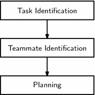
Challenges in establishing ad hoc teamwork
Fictitious play is a common approach used for learning in games [20]. In the classical fictitious play setting, agents play best response strategies against fixed strategy opponents.
For \(0<n<N\), we define
$$\begin{aligned} \hat{V}(h_{1:n},a_{-\alpha })=\frac{1}{n}\sum _{t=1}^{n}U_{T^*}(\left\langle a_\alpha (t),a_{-\alpha }\right\rangle ). \end{aligned}$$For \(n=0\) and for all \(a_{-\alpha }\in \mathcal {A}_{-\alpha }\), we define \(\hat{V}(h_{1:n},a_{-\alpha })=\hat{V}(h_0,a_{-\alpha })=0\).
These teammates are also known as memory-bounded best response agents.
For \(n<N\), we extend the definition as in footnote 4.
These are two distinct goals, and both must be reflected in the POMDP formulation. While the former seeks to identify the target task, the latter seeks to play that task as well as possible.
In our implementation, the RL agent runs the standard \(Q\)-learning algorithm with a fixed learning rate of \(\alpha =0.2\). The value for \(\alpha \) was empirically selected to maximize the learning performance of the agent. Additionally, exploration is ensured using a greedy policy combined with optimistic initialization of the \(Q\)-values, as discussed in the classical book of Sutton and Barto [62].
We recall that low values of \(\gamma \) indicate the MDP agent that payoffs arriving sooner are more valuable than payoffs arriving later.
We recall that, except for the RL agent, the results presented merely quantify the payoff that the agents would obtain from their action choices. At runtime, no payoff is granted to the agents, i.e., payoff information is not available for learning.
Table 3 Performance of the different approaches in the e-commerce scenario for different horizon lengths. The results are averages over \(1,000\) independent Monte Carlo runs The learning time can be observed from the plots in Fig. 8. It corresponds (roughly) to the number of time steps needed for the slope of the learning curve to stabilize. For \(H=1\), the learning time is \({\sim }16\) time steps, while for \(H=3\), the learning time is \({\sim }90\).
The generation of the payoff matrices was done by generating each entry uniformly at random in the range \([-300;500]\).
We emphasize that the reported times are offline planning times. The online learning approach requires no offline planning and hence no time is reported for that approach. All times were obtained in a computer equipped with a 3.0 GHz dual core processor and 16Gb of RAM.
With 2-action agents and \(H=2\), the total number of states is \(2^{20}\).
A toroidal grid world consists of a finite grid such that, if an agent “exits” one of the edges of the grid, it “re-enters” at the opposite edge. For example, if the agent moves right at the right edge of the environment, it will re-enter at the left edge of the environment, as seen in the diagram below:

In this context, we refer to a “mistake” as an action that is not a best response to the actions of the ad hoc agent.
Note that, by construction, the family \(\left\{ \mathcal {F}_n,n=1,\ldots \right\} \) is a non-increasing family of \(\sigma \)-algebras.


References
Abbeel, P. (2008). Apprenticeship learning and reinforcement learning with application to robotic control. PhD thesis, Stanford University.
Agmon, N., & Stone, P. (2012). Leading ad hoc agents in joint action settings with multiple teammates. In Proceedings 11th International Conference on Autonomous Agents and Multiagent Systems (pp. 341–348).
Albrecht, S., & Ramamoorthy, S. (2013). A game-theoretic model and best-response learning method for ad hoc coordination in multiagent systems. In: Proceedings 2013 International Conference on Autonomous Agents and Multiagent Systems (pp. 1155–1156).
Barrett, S., & Stone, P. (2011). Ad hoc teamwork modeled with multi-armed bandits: An extension to discounted infinite rewards. In Proceedings of 2011 AAMAS Workshop on Adaptive and Learning Agents (pp. 9–14).
Barrett, S., & Stone, P. (2012). An analysis framework for ad hoc teamwork tasks. In Proceedings of 11th International Conference on Autonomous Agents and Multiagent Systems (pp. 357–364).
Barrett, S., Stone, P., & Kraus, S. (2011). Empirical evaluation of ad hoc teamwork in the pursuit domain. In Proceedings of 10th International Conference on Autonomous Agents and Multiagent Systems (pp. 567–574).
Barrett, S., Stone, P., Kraus, S., & Rosenfeld, A. (2013). Teamwork with limited knowledge of reammates. In Proceedings of 27th AAAI Conference on Artificial Intelligence.
Barron, A. (1988). The exponential convergence of posterior probabilities with implications for Bayes estimators of density functions. Technical Report 7, University of Illinois at Urbana-Champaign.
Blackwell, D., & Dubbins, L. (1962). Merging of opinions with increasing information. The Annals of Mathematical Statistics, 33(3), 882–886.
Boutilier, C. (1996). Planning, learning and coordination in multiagent decision processes. In Proceedings 6th Conference on Theoretical Aspects of Rationality and Knowledge (pp. 195–210).
Bowling, M., & McCracken, P. (2005). Coordination and adaptation in impromptu teams. In Proceedings of 20th AAAI Conference on Artificial Intelligence (pp. 53–58).
Cesa-Bianchi, N., & Lugosi, G. (2006). Prediction, learning and games. New York: Cambridge University Press.
Chakraborty, D., & Stone, P. (2013). Cooperating with a Markovian ad hoc teammate. In Proceedings of 12th International Conference on Autonomous Agents and Multiagent Systems (pp. 1085–1092).
Clarke, B., & Barron, A. (1990). Information-theoretic asymptotics of Bayes methods. IEEE Transactions on Information Theory, 36(3), 371–453.
de Farias, D., & Megiddo, N. (2006). Combining expert advice in reactive environments. The Journal of the ACM, 53(5), 762–799.
Duff, M. (2002). Optimal learning: Computational procedures for Bayes-adaptive Markov decision processes. PhD thesis, University of Massassachusetts Amherst.
Fu, J., & Kass, R. (1988). The exponential rates of convergence of posterior distributions. Annals of the Institute of Statistical Mathematics, 40(4), 683–691.
Fudenberg, D., & Levine, D. (1989). Reputation and equilibrium selection in games with a patient player. Econometrica, 57(4), 759–778.
Fudenberg, D., & Levine, D. (1993). Steady state learning and Nash equilibrium. Econometrica, 61(3), 547–573.
Fudenberg, D., & Levine, D. (1998). The theory of learning in games. Cambridge, MA: MIT Press.
Ganzfried, S., & Sandholm, T. (2011). Game theory-based opponent modeling in large imperfect-information games. In Proceedings of 10th International Conference on Autonomous Agents and Multiagent Systems (pp. 533–540).
Genter, K., Agmon, N., & Stone, P. (2011). Role-based ad hoc teamwork. In Proceedings of 25th AAAI Conference on Artificial Intelligence (pp. 1782–1783).
Genter, K., Agmon, N., & Stone, P. (2013). Ad hoc teamwork for leading a flock. In Proceedings of 12th International Conference on Autonomous Agents and Multiagent Systems (pp. 531–538).
Ghosal, S., & van der Vaart, A. (2007). Convergence rates of posterior distributions for non IID observations. The Annals of Statistics, 35(1), 192–223.
Ghosal, S., Ghosh, J., & van der Vaart, A. (2000). Convergence rates of posterior distributions. The Annals of Statistics, 28(2), 500–531.
Gittins, J. (1979). Bandit processes and dynamic allocation indices. Journal of the Royal Statistical Society B, 41(2), 148–177.
Gmytrasiewicz, P., & Doshi, P. (2005). A framework for sequential planning in multiagent settings. Journal of Artificial Intelligence Research, 24, 49–79.
Gossner, O., & Tomala, T. (2008). Entropy bounds on Bayesian learning. Journal of Mathematical Economics, 44, 24–32.
Haussler, D., & Opper, M. (1997). Mutual information, metric entropy and cumulative entropy risk. Annals of Statistics, 25(6), 2451–2492.
Hoeffding, W. (1963). Probability inequalities for sums of bounded random variables. Journal of the American Statistical Association, 58, 13–30.
Jordan, J. (1991). Bayesian learning in normal form games. Games and Economic Behavior, 3, 60–81.
Jordan, J. (1992). The exponential convergence of Bayesian learning in normal form games. Games and Economic Behavior, 4(2), 202–217.
Kaelbling, L., Littman, M., & Cassandra, A. (1998). Planning and acting in partially observable stochastic domains. Artificial Intelligence, 101, 99–134.
Kalai, E., & Lehrer, E. (1993). Rational learning leads to Nash equilibrium. Econometrica, 61(5), 1019–1045.
Kauffman, E., Cappé, O., & Garivier, A (2012). On Bayesian upper confidence bounds for bandit problems. In Proceedings of 15th International Conference on Artificial Intelligence and Statistics (pp. 592–600).
Kauffman, E., Korda, N., & Munos, R. (2012). Thompson sampling: An asymptotically optimal finite-time analysis. In Proceedings of 23rd International Conference on Algorithmic Learning Theory (pp. 199–213).
Kautz, H., Pelavin, R., Tenenberg, J., & Kaufmann, M. (1991). A formal theory of plan recognition and its implementation. Reasoning about plans (pp. 69–125). San Mateo, CA: Morgan Kaufmann.
Kocsis, L., & Szepesvári, C. (2006). Bandit based Monte-Carlo planning. In Proceedings of 17th European Conference on Machine Learning (pp. 282–293).
Lai, T., & Robbins, H. (1985). Asymptotically efficient adaptive allocation rules. Advances in Applied Mathematics, 6(1), 4–22.
Leyton-Brown, K., & Shoham, Y. (2008). Essential of game theory: A concise, multidisciplinary introduction. San Rafael, CA: Morgan & Claypool Publishers.
Liemhetcharat, S., & Veloso, M. (2014). Weighted synergy graphs for effective team formation with heterogeneous ad hoc agents. Artificial Intelligence, 208, 41–65.
Littman, M. (2001). Value-function reinforcement learning in Markov games. Journal of Cognitive Systems Research, 2(1), 55–66.
Madani, O., Hanks, S., & Condon, A. (1999). On the undecidability of probabilistic planning and infinite-horizon partially observable Markov decision problems. In Proceedings of 16th AAAI Conference Artificial Intelligence (pp. 541–548).
Nachbar, J. (1997). Prediction, optimization and learning in repeated games. Econometrica, 65(2), 275–309.
Ng, A., & Russel, S. (2000). Algorithms for inverse reinforcement learning. In Proceedings of 17th International Conference on Machine Learning (pp. 663–670).
Pineau, J., Gordon, G., & Thrun, S. (2006). Anytime point-based approximations for large POMDPs. Journal of Artificial Intelligence Research, 27, 335–380.
Poupart, P., Vlassis, N., Hoey, J., & Regan, K. (2006). An analytic solution to discrete Bayesian reinforcement learning. In Proceedings of 23rd International Conference on Machine Learning (pp. 697–704).
Pourmehr, S., & Dadkhah, C. (2012). An overview on opponent modeling in RoboCup soccer simulation 2D. Robot soccer world cup XV (pp. 402–414). Berlin: Springer.
Puterman, M. (2005). Markov decision processes: Discrete stochastic dynamic programming. New York: Wiley.
Ramchurn, S., Osborne, M., Parson, O., Rahwan, T., Maleki, S., Reece, S., Huynh, T., Alam, M., Fischer, J., Rodden, T., Moreau, L., & Roberts, S. (2013). AgentSwitch: Towards smart energy tariff selection. In Proceedings of 12th International Conference on Autonomous Agents and Multiagent Systems (pp. 981–988).
Rosenthal, S., Biswas, J., & Veloso, M. (2010). An effective personal mobile robot agent through symbiotic human-robot interaction. In Proceedings of 9th International Conference on Autonomous Agents and Multiagent Systems (pp. 915–922).
Seuken, S., & Zilberstein, S. (2008). Formal models and algorithms for decentralized decision making under uncertainty. Journal of Autonomous Agents and Multiagent Systems, 17(2), 190–250.
Shani, G., Pineau, J., & Kaplow, R. (2013). A survey of point-based POMDP solvers. Journal of Autonomous Agents and Multiagent Systems, 27(1), 1–51.
Shen, X., & Wasserman, L. (2001). Rates of convergence of posterior distributions. The Annals of Statistics, 29(3), 687–714.
Shiryaev, A. (1996). Probability. New York: Springer.
Spaan, M., & Vlassis, N. (2005). Perseus: Randomized point-based value iteration for POMDPs. Jornal of Artificial Intelligence Reseasrch, 24, 195–220.
Spaan, M., Gordon, G., & Vlassis, N. (2006). Decentralized planning under uncertainty for teams of communicating agents. In Proceedings of 5th International Conference on Autonomous Agents and Multi Agent Systems (pp. 249–256).
Stone, P., & Kraus, S. (2010). To teach or not to teach? Decision-making under uncertainty in ad hoc teams. In Proceedings of 9th International Conference on Autonomous Agents and Multiagent Systems (pp. 117–124).
Stone, P., & Veloso, M. (2000). Multiagent systems: A survey from a machine learning perspective. Autonomous Robots, 8(3), 345–383.
Stone, P., Kaminka, G., Kraus, S., & Rosenschein, J. (2010). Ad hoc autonomous agent teams: Collaboration without pre-coordination. In Proceedings of 24th AAAI Conference on Artificial Intelligence (pp. 1504–1509).
Stone, P., Kaminka, G., & Rosenschein, J. (2010). Leading a best-response teammate in an ad hoc team. Agent-mediated electronic commerce. Designing trading strategies and mechanisms for electronic markets. Lecture notes in business information processing (pp. 132–146). Berlin: Springer.
Sutton, R., & Barto, A. (1998). Reinforcement learning: An introduction. Cambridge, MA: MIT Press.
Walker, S., Lijoi, A., & Prünster, I. (2007). On rates of convergence for posterior distributions in infinite-dimensional models. The Annals of Statistics, 35(2), 738–746.
Wang, X., & Sandholm, T. (2002). Reinforcement learning to play an optimal Nash equilibrium in team Markov games. Advances in Neural Information Processing Systems, 15, 1571–1578.
Watkins, C. (1989). Learning from delayed rewards. PhD thesis, King’s College, Cambridge Univ.
Wu, F., Zilberstein, S., & Chen, X. (2011). Online planning for ad hoc autonomous agent teams. In Proceedings of 22nd International Joint Conference on Artificial Intelligence (pp. 439–445).
Yorke-Smith, N., Saadati, S., Myers, K., & Morley, D. (2012). The design of a proactive personal agent for task management. International Journal on Artificial Intelligence Tools, 21(1), 90–119.
Acknowledgments
The authors gratefully acknowledge the anonymous reviewers for the many useful suggestions that greatly improved the clarity of the presentation. This work was partially supported by national funds through Fundação para a Ciência e a Tecnologia (FCT) with reference UID/CEC/50021/2013 and the Carnegie Mellon Portugal Program and its Information and Communications Technologies Institute, under Project CMUP-ERI/HCI/0051/2013.
Author information
Authors and Affiliations
Corresponding author
Electronic supplementary material
Below is the link to the electronic supplementary material.
Supplementary material 1 (m4v 14596 KB)
Appendix: Proofs
Appendix: Proofs
In this appendix, we collect the proofs of the different statements introduced in the main text.
1.1 Proof of Theorem 1
In our proof, we use the following auxiliary result, which is a simple extension of Lemma 2.3 in [12].
Lemma 1
For all \(N\ge 2\), for all \(\beta \ge \alpha \ge 0\) and for all \(d_1,\ldots ,d_N\ge 0\) such that
let
Then, for all \(x_1,\ldots ,x_N\),
where \(X\) is a r.v. taking values in \(\left\{ x_1,\ldots ,x_N\right\} \) and such that \(\mathbb {P}_{}\left[ X=x_i\right] =q_i\).
Proof
We have
where \(D\) is a r.v. taking values in \(\left\{ d_1,\ldots ,d_N\right\} \) such that \(\mathbb {P}_{}\left[ D=d_i\right] =q_i\), and the last inequality follows from Jensen’s inequality. Since \(D\) takes at most \(N\) values, we have that
where \(H(D)\) is the entropy of the r.v. \(D\), and hence
Finally, because \(\beta \ge \alpha \), we can replace (18) in (17) to get
\(\square \)
We are now in a position to prove Theorem 1. Let \(h_{1:n}\) be a fixed history. Define \(\gamma _0=0\) and, for \(t\ge 0\), let
Using the notation above, we have that
Our proof closely follows the proof of Theorem 2.2 of [12]. We establish our result by deriving upper and lower bounds for the quantity \(\ln (W_n/W_0)\).
On the one hand,
Becayse \(w_t(\tau )>0\) for all \(t\), then for any \(\tau \in \mathcal {T}\),
On the other hand, for \(t>1\),
Using Lemma 1, we can write
where the last equality follows from the definition of \(P\). Noting that
we can set the upper bound \(\ln (W_n/W_0)\) as
The fact that \(\gamma _{t+1}<\gamma _t\) for all \(t\ge 1\) further implies
Replacing the definition of \(\gamma _n\) in the first term, we get
Finally, putting together (19) and (20) yields
or, equivalently,
Because the above inequality holds for all \(\tau \),
\(\square \)
1.2 Proof of Theorem 2
Our proof involves three steps:
-
In the first step, we show that, asymptotically, the ability of the ad hoc to predict future plays, given its initial belief over the target task, converges to that of an agent knowing the target task.
-
In the second step, we derive an upper bound for the regret that depends linearly on the relative entropy between the probability distribution over trajectories conditioned on knowing the target task and the probability distribution over trajectories conditioned on the prior over tasks.
-
Finally, in the third step, we use an information-theoretic argument to derive an upper bound to the aforementioned relative entropy, using the fact that the ad hoc agent is asymptotically able to predict future plays as well as if it knew the target task.
The proof is somewhat long and requires some notation and a number of auxiliary results, which are introduced in the continuation.
1.2.1 Preliminary results and notation
In this section, we introduce several preliminary results that will be of use in the proof. We start with a simple lemma due to Hoeffding [30] that provides a useful bound for the moment generating function of a bounded r.v. \(X\).
Lemma 2
Let \(X\) be a r.v. such that \(\mathbb {E}_{}\left[ X\right] =0\) and \(a\le X\le b\) almost surely. Then, for any \(\lambda >0\),
The following is a classical result from P. Levy [55, Theorem VII.3]. This result plays a fundamental role in establishing that the beliefs of the ad hoc agent asymptotically concentrate around the target task.
Lemma 3
Let \((\Omega , \mathcal {F}, \mathbb {P})\) be a probability space, and let \(\left\{ \mathcal {F}_n,n=1,\ldots \right\} \) be a non-decreasing family of \(\sigma \)-algebras, \(\mathcal {F}_1\subseteq \mathcal {F}_2\subseteq \ldots \subseteq \mathcal {F}\). Let \(X\) be a r.v. with \(\mathbb {E}_{}\left[ \left|X\right|\right] <\infty \) and let \(\mathcal {F}_\infty \) denote the smallest \(\sigma \)-algebra such that \(\bigcup _n\mathcal {F}_n\subseteq \mathcal {F}_\infty \). Then,
with probability 1.
We conclude this initial subsection by establishing several simple results. We write \(\mathbb {E}_{p}\left[ \cdot \right] \) to denote the expectation with respect to the distribution \(p\) and \(\mathrm {D_{KL}}\left( p\Vert q\right) \) to denote the Kullback-Liebler divergence (or relative entropy) between distributions \(p\) and \(q\), defined as
It is a well-known information-theoretic result (known as the Gibbs inequality) that \(\mathrm {D_{KL}}\left( p\Vert q\right) \ge 0\).
Lemma 4
Let \(X\) be a r.v. taking values in a discrete set \(\mathcal {X}\) and let \(p\) and \(q\) denote two distributions over \(\mathcal {X}\). Then, for any function  ,
,
Proof
Define, for \(x\in \mathcal {X}\),
Clearly, \(v(x)\ge 0\) and \(\sum _xv(x)=1\), so \(v\) is a distribution over \(\mathcal {X}\). We have
Because \(\mathrm {D_{KL}}\left( q\Vert v\right) \ge 0\),
and the result follows.\(\square \)
Lemma 5
(Adapted from [28]) Let \(\left\{ a_n\right\} \) be a bounded sequence of non-negative numbers. Then, \(\lim _na_n=0\) if and only if
Proof
Let \(A=\sup _na_n\) and, given \(\varepsilon >0\), define the set

By definition, \(\lim _na_n=0\) if and only if \(\left|M_\varepsilon \right|<\infty \) for any \(\varepsilon \). Let \(M_\varepsilon ^n=M_\varepsilon \cap \left\{ 1,\ldots ,n\right\} \). We have that
The conclusion follows.\(\square \)
1.2.2 Convergence of predictive distributions
We can now take the first step in establishing the result in Theorem 2. In particular, we show that, asymptotically, the ability of the ad hoc agent to predict future actions of the teammate player converges to that of an agent that knows the target task.
We start by noting that given the POMDP policy computed by Perseus and the initial belief for the ad hoc agent, it is possible to determine the probability of occurrence of any particular history of (joint) actions \(h\in \mathcal {H}\). In particular, we write
and
to denote the distribution over histories induced by the POMDP policy when the initial belief over tasks is, respectively, \(p_0\) and \(\delta _{\tau ^*}\). We write \(\delta _{\tau }\) to denote the belief over tasks that is concentrated in a single task \(\tau \). Note that, for a particular history \(h_{1:n}=\left\{ a(1),\ldots ,a(n)\right\} \), we can write
where \(B(h_{1:t-1},p_0)\) denotes the belief \(p_{t-1}\) over tasks computed from the initial belief \(p_0\) and the history \(h_{1:t-1}\). Let \(\mathcal {F}_n\) denote the \(\sigma \)-algebra generated by the history up to time-step \(n\), i.e., the smallest \(\sigma \)-algebra that renders \(H(n)\) measurable.Footnote 18 The assertion we seek to establish is formalized as the following result.
Proposition 1
Suppose that \(p_0(T^*)>0\), i.e., the initial belief of the agent over tasks does not exclude the target task. Then, with probability 1 (w.p.1), for every \(\varepsilon >0\), there is \(N>0\) such that, for every \(m\ge n\ge N\),
Proof
Given a history \(h'\) of length \(n\), let \(\mathcal {H}_{\mid h'}\) denote the subset of \(\mathcal {H}\) that is compatible with \(h'\), i.e., the set of histories \(h\in \mathcal {H}\) such that \(h_{1:n}=h'\). Our proof goes along the lines of [34]. We start by noticing that, because \(p_0(T^*)>0\), it holds that
i.e., \(\mu \ll \tilde{\mu }\) (\(\mu \) is absolutely continuous w.r.t. \(\tilde{\mu }\)). We can thus define, for every finite history \(h\), a function  as
as
with \(d(h)=0\) if \(\mu (h)=0\). From Lemma 3,
which is an \(\mathcal {F}_{\infty }\)-measurable and strictly positive random variable. On the other hand, by definition, we have that
We now note that, for \(m\ge n, \mu (H(m)\mid H(n))\) is a r.v. such that
with a similar relation holding for \(\tilde{\mu }(H(m)\mid H(n))\). From (21), \(\mathbb {E}_{\tilde{\mu }}\left[ d(H(m))\mid \mathcal {F}_n\right] \) converges w.p.1 to a strictly positive r.v. Then, for any \(\varepsilon >0\), there is \(N(\varepsilon )>0\) such that, for \(m\ge n\ge N\),
Combining (22) with (23), we finally get that, for any \(\varepsilon >0\), there is \(N(\varepsilon )>0\) such that, for \(m\ge n\ge N\), w.p.1,
and the proof is complete.\(\square \)
1.2.3 Initial upper bound
We now proceed by deriving an upper bound to the regret of any POMDP policy that depends on the relative entropy between the distributions \(\mu \) and \(\tilde{\mu }\), defined in ‘Convergence of predictive distributions section’ under Appendix 2. This bound will later be improved to finally yield the desired result.
Proposition 2
Suppose that \(p_0(T^*)>0\), i.e., the initial belief of the agent over tasks does not exclude the target task. Then,
Proof
The expected reward received by following the POMDP policy from the initial belief \(\delta _{\tau ^*}\) is given by
Similarly, for the initial belief \(p_0\), we have
Using Lemma 4,
Simple computations yield
Because the exponential is a convex function, we can write
Applying Lemma 2 to the second term on the right-hand side and replacing the definitions of \(J_P\) and \(J_{\tau ^*}\) yields
and the proof is complete.\(\square \)
1.2.4 Refined upper bound
We can now establish the result in Theorem 2. We use Lemma 5 and Proposition 1 to derive an upper bound for the term \(\mathrm {D_{KL}}\left( \mu (H(n))\Vert \tilde{\mu }(H(n))\right) \), which appears in Proposition 2. The conclusion of Theorem 2 immediately follows.
Proposition 3
Suppose that \(p_0(T^*)>0\), i.e., the initial belief of the agent over tasks does not exclude the target task. Then, the sequence \(\left\{ d_n\right\} \) defined, for each \(n\), as
is \(o(n)\).
Proof
We start by noting that
which implies that
For each  , define the sequences \(\left\{ a_n\right\} , \left\{ b_n\right\} \) and \(\left\{ c_n\right\} \) as
By construction, we have \(a_n>0\) and \(b_n>0\) for all  . Additionally, from Proposition 1,
w.p.1, implying that \(\lim _nc_n=0\) w.p.1. By Lemma 5, we have that, w.p.1,
which finally yields that
and the proof is complete.\(\square \)
Rights and permissions
About this article

Cite this article
Melo, F.S., Sardinha, A. Ad hoc teamwork by learning teammates’ task. Auton Agent Multi-Agent Syst 30, 175–219 (2016). https://doi.org/10.1007/s10458-015-9280-x
Published:
Issue Date:
DOI: https://doi.org/10.1007/s10458-015-9280-x