Space-time Generalized Riemann Problem Solvers of Order k for Linear Advection with Unrestricted Time Step

Abstract

This work concerns high-order approximations of the linear advection equation in very long time. A GRP-type scheme of arbitrary high-order in space and time with no restriction on the time step is developed. In the usual GRP solvers, we consider a polynomial approximation of the solution in space in each cell at the initial time. Here, we add a second polynomial approximation of the solution in time in each interface. Thanks to this double approximation, the resulting scheme is compact. It is proved to be of order k+1 in space and time, where k is the degree of the polynomials. Thanks to the compactness of the scheme, a two-dimensional extension is detailed on unstructured meshes made of triangles. Several numerical test-cases and comparison with existing methods illustrate the excellent behaviour of the scheme.

Appendix

Evolution Step

Case two targets (explicit):

• ∘ We know the solution $u_{i}^{n}(x,y)$ in the cell T _i at time t ⁿ and the solution $v_{j3}^{n+\frac{1}{2}}(t,\omega)$ on the interface $I_{j3}^{n+\frac{1}{2}}$ .

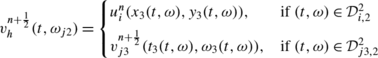
• ∘ We define θ ₁ as the intersection between the characteristic line coming from $s_{j3}^{n}$ and the segment $s_{j1}^{n+1}$. We also define θ ₂, the intersection between the characteristic line coming from $s_{j3}^{n}$ and the segment $s_{j2}^{n+1}$. Then we call M ₁ the projection of θ ₁ on $s_{j1}^{n}$ and M ₂ the projection of θ ₂ on $s_{j2}^{n}$ (see Fig. 21).

  Fig. 21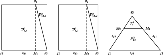

  

  Incoming solutions on the interface (left) and on the cell (right) for the explicit case two targets

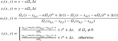
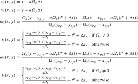
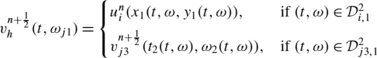
• ∘ The exact solution on the cell T _i at time t ⁿ⁺¹ is:

  

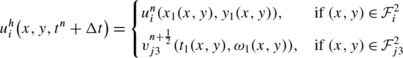
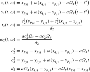
  with:

  

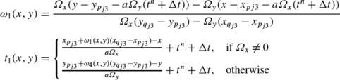
• ∘ The exact solution on the interface $I_{j1}^{n+\frac{1}{2}}$ is:

  

  with:

  

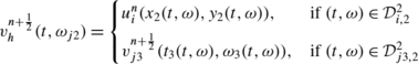
• ∘ The exact solution on the interface $I_{j2}^{n+\frac{1}{2}}$ is:

  

  with:

  

Case one target (explicit):

• ∘ We know the solution $u_{i}^{n}(x,y)$ in the cell T _i at time t ⁿ and the solutions $v_{j1}^{n+\frac{1}{2}}(t,\omega)$ and $v_{j2}^{n+\frac{1}{2}}(t,\omega)$ on the interfaces I _j1 and $I_{j2}^{n+\frac{1}{2}}$.

• ∘ We define θ ₁ as the intersection between the characteristic line coming from the segment $s_{j1}^{n}$ and the segment $s_{j3}^{n+1}$ (i.e. such that $d(s_{j3}^{n},s_{j1}^{n}) = a \Delta t$). We also define θ ₂ as the intersection between the characteristic line coming from the segment $s_{j2}^{n}$ and the segment $s_{j3}^{n+1}$ (i.e. such that $d(s_{j3}^{n},s_{j2}^{n}) = a \Delta t$). Then we call M ₁ the projection of θ ₁ on $s_{j3}^{n}$ and M ₂ the projection of θ ₂ on $s_{j3}^{n}$ (see Fig. 22).

  Fig. 22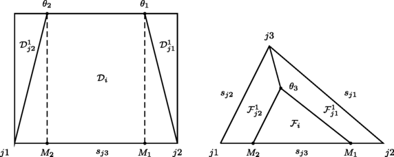

  

  Incoming solutions on the interface (left) and on the cell (right) for the explicit case 1

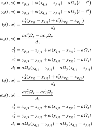
• ∘ The exact solution on the cell T _i at time t ⁿ⁺¹ is:

  

  with:

  

• ∘ The exact solution on the interface $I_{j3}^{n+\frac{1}{2}}$ is:

  

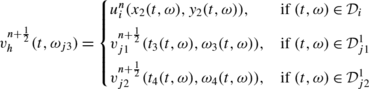
  with:

  

Case two targets (implicit):

• ∘ We know the solution $u_{i}^{n}(x,y)$ in the cell T _i at time t ⁿ and the solution $v_{j3}^{n+\frac{1}{2}}(t,\omega)$ on the interface $I_{j3}^{n+\frac{1}{2}}$ .

• ∘ We define θ ₃ as the intersection between the characteristic line coming from $s_{j3}^{n}$ and the segment [t ⁿ,t ⁿ⁺¹] for (x,y)=(x _j3,y _j3) (see Fig. 23).

  Fig. 23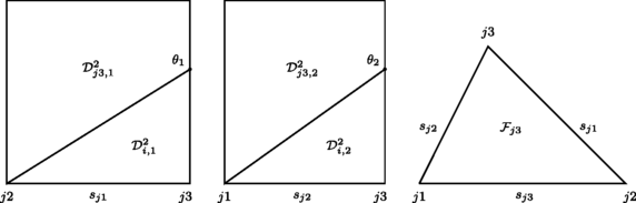

  

  Incoming solutions on the interface (left) and on the cell (right) for the implicit case 2

• ∘ The exact solution on the cell T _i at time t ⁿ⁺¹ is:

  

  with:

  

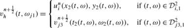
• ∘ The exact solution on the interface $I_{j1}^{n+\frac{1}{2}}$ is:

  

  with:

  

• ∘ The exact solution on the interface $I_{j2}^{n+\frac{1}{2}}$ is:

  

  with:

  

Projection Step

The exact solutions are respectively projected onto the spaces $\mathbb {P}^{k}_{C}$ and $\mathbb {P}^{k}_{I}$: in the cell T _i at time t ⁿ⁺¹, the exact solution is projected in $\mathbb {P}^{k}_{C}$, and on the interfaces $I_{j}^{n+\frac{1}{2}}$, the solution is projected in $\mathbb {P}^{k}_{I}$. For the case n^∘1 explicit, this leads to the two minimization problems:

(20)

(21)

for the case n^∘2 explicit, it leads to the three minimization problems:

(22)

(23)

(24)

and for the case explicit two targets, it also leads to three minimization problems:

(25)

(26)

(27)

Thanks to the Petrov-Galerkin conditions, we can rewrite (20), (21) as:

(28)

(29)

and (22)–(24) as:

(30)

(31)

(32)

Using the decomposition of the solutions in their corresponding basis:

the minimization problems (28), (29) are equivalent to solving the two following linear systems of size $\frac{(k+1)(k+2)}{2}$:

and (30)–(32) are equivalent to solving three linear systems of size $\frac{(k+1)(k+2)}{2}$:

The matrices are the same that in the case n^∘1 implicit and the case n^∘2 explicit. For the right hand sides, we have first for the case n^∘1 explicit:

then for the case n^∘2 implicit:

and for the case explicit two targets:

where the coefficients are given by:

References

Abgrall, R., Mezine, M.: Construction of second order accurate monotone and stable residual distribution schemes for unsteady flow problems. J. Comput. Phys. 188, 16–55 (2003)
Abgrall, R., Deconinck, H., Ricchiuto, M., Villedieu, N.: On uniformly high-order accurate residual distribution schemes for advection-diffusion. J. Comput. Appl. Math. 215(2), 547–556 (2008)
Abgrall, R., Larat, A., Ricchiuto, M., Tavé, C.: A simple construction of very high order non oscillatory compact schemes on unstructured meshes. Comput. Fluids 38(7), 1314–1323 (2009)
Ben-Artzi, M., Birman, A.: Application of the generalized Riemann problem method to 1-D compressible flows with material interfaces. J. Comput. Phys. 65(1), 170–178 (1986)
Ben-Artzi, M., Falcovitz, J.: Recent developments of the GRP method. JSME Int. J. Ser. B Fluids Therm. Eng. 38(4), 497–517 (1995)
Ben-Artzi, M., Falcovitz, J.: Generalized Riemann Problems in Computational Fluid Dynamics. Cambridge Monographs on Applied and Computational Mathematics. (2003)
Ben-Artzi, M., Li, J., Warnecke, G.: A direct Eulerian GRP scheme for compressible fluid flows. J. Comput. Phys. 218, 19–43 (2006)
Berthon, C., Turpault, R.: Asymptotic preserving HLL schemes. Numer. Methods Partial Differ. Equ. 27(6), 1396–1422 (2011)
Chalons, C., Coquel, F., Godlewski, E., Raviart, P.A., Seguin, N.: Godunov-type schemes for hyperbolic systems with parameter dependent source. The case of Euler system with friction. Math. Models Methods Appl. Sci. 20(11), 2109 (2010)
Chandrasekhar, S.: Radiative Transfer. Dover, New York (1950)
Cockburn, B., Shu, C.W.: TVD Runge-Kutta local projection discontinuous Galerkin finite element method for scalar conservation laws II: general framework. Math. Comput. 52, 411 (1989)
Cockburn, B., Shu, C.W.: The Runge-Kutta discontinuous Galerkin method for conservation laws V: multidimensional systems. J. Comput. Phys. 141(2), 199–224 (1998)
Dai, W.W., Woodward, P.R.: Moment preserving schemes for Euler equations. Comput. Fluids 46, 186–196 (2011)
Davidson, B.: Neutron Transport Theory. Clarendon, Oxford (1957)
Degond, P., Pareschi, L., Russo, G.: Modeling and Computational Methods for Kinetic Equations. Birkhäuser, Basel (2004)
Dumbser, M., Käser, M.: Arbitrary high order non-oscillatory finite volume schemes on unstructured meshes for linear hyperbolic systems. J. Comput. Phys. 221(2), 693–723 (2007)
Dumbser, M., Munz, C.D.: Arbitrary high-order discontinuous Galerkin schemes. In: Numerical Methods for Hyperbolic and Kinetic Problems, pp. 295–333 (2005)
Dumbser, M., Zanotti, O.: Very high order PNPM schemes on unstructured meshes for the resistive relativistic MHD equations. J. Comput. Phys. 228(18), 6991–7006 (2009)
Dumbser, M., Balsara, D., Munz, C.D., Toro, E.F.: A unified framework for the construction of one-step finite-volume and discontinuous Galerkin schemes on unstructured meshes. J. Comput. Phys. 227(18), 8209–8253 (2008)
Dumbser, M., Enaux, C., Toro, E.F.: Finite volume schemes of very high order of accuracy for Stiff hyperbolic balance laws. J. Comput. Phys. 227(8), 3971–4001 (2008)
Filbet, F., Jin, S.: An asymptotic preserving scheme for the ES-BGK model of the Boltzmann equation. J. Sci. Comput. 46, 204–224 (2011)
Frénod, E., Salvarani, F., Sonnendrücker, E.: Long time simulation of a beam in a periodic focusing channel via a two-scale PIC-method. Math. Models Methods Appl. Sci. 19(2), 175–197 (2009)
Gassner, G., Dumbser, M., Hindenlang, F., Munz, C.D.: Explicit one-step time discretizations for discontinuous Galerkin and finite volume schemes based on local predictors. J. Comput. Phys. 230, 4232–4247 (2011)
Glassey, R.T.: The Cauchy Problem in Kinetic Theory. SIAM, Philadelphia (1996)
Glimm, J., Marshall, G., Plohr, B.: A generalized Riemann problem for quasi-one-dimensional gas flows. Adv. Appl. Math. 5(1), 1–30 (1984)
Gosse, L., Toscani, G.: Asymptotic-preserving & well-balanced schemes for radiative transfer and the Rosseland approximation. Numer. Math. 98, 223–250 (2003)
Gottlieb, S., Shu, C.W.: Total variation diminishing Runge-Kutta schemes. Math. Comput. 67, 73–85 (1998)
Harten, A., Engquist, B., Osher, S., Chakravarthy, S.R.: Uniformly high-order accurate essentially non-oscillatory schemes, III. J. Comput. Phys. 71(2), 231–303 (1987)
Helffer, B., Nier, F.: Hypoelliptic Estimates and Spectral Theory for Fokker-Planck Operators and Witten Laplacians. Springer, Berlin (2005)
Hoteit, H., Ackerer, P., Mosé, R., Erhel, J., Philippe, B.: New two-dimensional slope limiters for discontinuous Galerkin methods on arbitrary meshes. Int. J. Numer. Methods Eng. 61(14), 2566–2593 (2004)
Jiang, G.S., Shu, C.W.: Efficient implementation of weighted ENO schemes. J. Comput. Phys. 126(1), 202–228 (1996)
Jin, S.: Efficient asymptotic-preserving (AP) schemes for some multiscale kinetic equations. SIAM J. Sci. Comput. 21, 441–454 (1999)
Klaij, C., van der Vegt, J.J.W., van der Ven, H.: Space-time discontinuous Galerkin method for the compressible Navier-Stokes equations. J. Comput. Phys. 217, 589–611 (2006)
Lemou, M., Mieussens, L.: Time implicit schemes and fast approximations of the Fokker-Planck-Landau equation. SIAM J. Sci. Comput. 27(3), 809–830 (2007)
LeVeque, R.J.: Finite Volume Methods for Hyperbolic Problems. Cambridge University Press, Cambridge (2002)
Liu, T.P., Osher, S., Chan, T.: Weighted essentially non-oscillatory schemes. J. Comput. Phys. 115, 200–212 (1994)
Lörcher, F., Gassner, G., Munz, C.D.: A discontinuous Galerkin scheme based on a space-time expansion. I. Inviscid compressible flow in one space dimension. J. Sci. Comput. 32(2), 175–199 (2007)
Lowrie, R.B., Roe, P.L., Van Leer, B.: A space-time discontinuous Galerkin method for the time accurate numerical solution of hyperbolic conservation laws. In: Proceedings of 12th AIAA CFD Conference, pp. 95–1658 (1995)
Mihalas, D., Weibel-Mihalas, B.: Foundations of Radiation Hydrodynamics. Dover, New York (1999)
Pomraning, G.C.: The Equations of Radiation Hydrodynamics. Pergamon, Elmsford (1973)
Toro, E.F.: Riemann Solvers and Numerical Methods for Fluid Dynamics. A Practical Introduction. Springer, Berlin (1999)
van der Vegt, J.J.W., van der Ven, H.: Space-time discontinuous Galerkin finite element method with dynamic grid motion for inviscid compressible flows I. General formulation. J. Comput. Phys. 182, 546–585 (2002)
Author information
Authors and Affiliations
Corresponding author