A Second-Order Boundary Condition Capturing Method for Solving the Elliptic Interface Problems on Irregular Domains

Abstract

A second-order boundary condition capturing method is presented for the elliptic interface problem with jump conditions in the solution and its normal derivative. The proposed method is an extension of the work in Liu et al. (J Comput Phys 160(1):151–178, 2000) to a higher order. The motivation of proposed method is that the approximated value at the interface can be reconstructed by proper interpolation based on the level set representation from Gibou et al. (J Comput Phys 176(1):205–227, 2002). A second-order accurate method is constructed, both in the solution and its gradient, using second-order finite difference approximation. Several numerical results demonstrate that the proposed method is indeed second-order accurate in the solution and its gradient in the $L^{2}$ and $L^{\infty }$ norms.

Appendix: Formulation of \(\mathbf {M}\) in (41)

The actual computation of the reduced $\mathbf {M}$ in (41) will herein be presented. We assume that $(x_{i},y_{j}) \in {\Omega }^-$. With the choice of $\mathbf {x_\text {ext}}$, the approximation of $\nabla u$ at the interface by quadratic interpolation satisfying (26) will be formulated explicitly.

Fig. 15

Illustration for interface and points of case 1

Fig. 16

Illustration for interface and points of case 2

• Case 1 The interface intersects one grid segment. Without loss of generality, we may assume that ${\mathbf {x}}_{\mathbf {R}}$ is not on the grid, and ${\mathbf {x}}_{\mathbf {T}},{\mathbf {x}}_{\mathbf {B}},{\mathbf {x}}_{\mathbf {L}}$ are on the grid, as shown in Fig. 15. We need only discretize the jump condition at ${\mathbf {x}}_{\mathbf {R}}=(x_{R},y_{j})$. At the remaining points, ${\mathbf {x}}_{\mathbf {T}},{\mathbf {x}}_{\mathbf {B}}$ and ${\mathbf {x}}_{\mathbf {L}}$, we have $u_T^-=u_{i,j+1},u_B^-=u_{i,j-1}$ and $u_L^-=u_{i-1,j}$. Let $\mathbf {x_\text {ext}}= (x_{i-1},y_{j-1})$. Using second-order finite differences in Cartesian directions (29) with $u_L^-= u_{i-1,j}$, we obtain

  $$\begin{aligned} \begin{aligned} u_x^+({\mathbf {x}}_{\mathbf {R}})&\approx \left. \left( -\frac{3-2\theta _R}{(1-\theta _R)(2-\theta _R)} u_R^+ +\frac{2-\theta _R}{1-\theta _R} u_{i+1,j}- \frac{1-\theta _R}{2-\theta _R} u_{i+2,j}\right) \bigg /\varDelta x \right. ,\\ u_x^-({\mathbf {x}}_{\mathbf {R}})&\approx \left. \left( \frac{\theta _R}{\theta _R+1} u_{i-1,j} - \frac{\theta _R+1}{\theta _R} u_{i,j}+ \frac{2\theta _R+1}{\theta _R(\theta _R+1)} u_{R}^- \right) \bigg / \varDelta x\right. . \end{aligned} \end{aligned}$$

  We approximate $u_y^-({\mathbf {x}}_{\mathbf {R}})$ by $P_y$, where P is obtained by quadratic interpolation (26).

  $$\begin{aligned} u_y^-({\mathbf {x}}_{\mathbf {R}})\approx \left. \left( \theta _R(u_{i,j}-u_{i-1,j}-u_{i,j-1}+u_{i-1,j-1}) +\frac{1}{2}(u_{i,j+1}-u_{i,j-1}) \right) \bigg / \varDelta y\right. . \end{aligned}$$

  $[\beta u_x]_R$ is discretized by equating the following relations:

  $$\begin{aligned} \begin{aligned} {[\beta u_n]}n_x -[\beta ](-u_x^- n_y + u_y^-n_x)n_y -\beta ^+[u]_\tau n_y = \beta ^+u_x^+ - \beta ^- u_x^- . \end{aligned} \end{aligned}$$

  $\mathbf {M}$ in (41) reduces to a $1\times 1$ matrix, and we may write system (41) as follows:

  $$\begin{aligned} \left( -\beta ^+\frac{3-2\theta _R}{(1-\theta _R)(2-\theta _r)}-(\beta ^- +[\beta ] n_y^2)\frac{2\theta _R+1}{\theta _R(\theta _R+1)} \right) u_R^- =\mathbf {N}\mathbf {u} + \mathbf {d}. \end{aligned}$$

• Case 2 The interface intersects two grid segment. We assume that $\phi _{i,j}\phi _{i+1,j}<0$ and $\phi _{i,j}\phi _{i,j+1}<0$. Thus, ${\mathbf {x}}_{\mathbf {R}}$ and ${\mathbf {x}}_{\mathbf {T}}$ are not on the grid, but ${\mathbf {x}}_{\mathbf {B}}$ and ${\mathbf {x}}_{\mathbf {L}}$ are on the grid. We choose $\mathbf {x_\text {ext}}$ to be $(x_{i-1},y_{j-1})$. The location of the interface and the choice of $\mathbf {x_\text {ext}}$ are shown in Fig. 16. As in case 1, we use second-order finite differences (29) and quadratic interpolation satisfying (26), and we approximate $u_x^+,u_x^-, u_y^-$ at ${\mathbf {x}}_{\mathbf {R}}$ and $u_y^+, u_y^-,u_x^-$ at ${\mathbf {x}}_{\mathbf {T}}$:

  $$\begin{aligned} \begin{aligned} u_x^+({\mathbf {x}}_{\mathbf {R}})&\approx \left. \left( -\frac{3-2\theta _R}{(1-\theta _R)(2-\theta _r)} u_R^+ +\frac{2-\theta _R}{1-\theta _R} u_{i+1,j}- \frac{1-\theta _R}{2-\theta _R} u_{i+2,j}\right) \bigg /\varDelta x \right. ,\\ u_x^-({\mathbf {x}}_{\mathbf {R}})&\approx \left. \left( \frac{\theta _R}{\theta _R+1} u_{i-1,j} - \frac{\theta _R+1}{\theta _R} u_{i,j}+ \frac{2\theta _R+1}{\theta _R(\theta _R+1)} u_{R}^- \right) \bigg / \varDelta x\right. ,\\ u_y^-({\mathbf {x}}_{\mathbf {R}})&\approx \left. \left( \theta _Ru_{xy}^0 + u_y^0 \right) \bigg / \varDelta y\right. \end{aligned} \end{aligned}$$

  and

  $$\begin{aligned} \begin{aligned} u_y^+({\mathbf {x}}_{\mathbf {T}})&\approx \left. \left( -\frac{3-2\theta _T}{(1-\theta _T)(2-\theta _T)} u_T^+ +\frac{2-\theta _T}{1-\theta _T} u_{i,j+1}- \frac{1-\theta _T}{2-\theta _T} u_{i,j+2}\right) \bigg /\varDelta y \right. ,\\ u_y^-({\mathbf {x}}_{\mathbf {T}})&\approx \left. \left( \frac{\theta _T}{\theta _T+1} u_{i,j-1} - \frac{\theta _T+1}{\theta _T} u_{i,j}+ \frac{2\theta _T+1}{\theta _T(\theta _T+1)} u_{T}^- \right) \bigg / \varDelta y\right. ,\\ u_x^-({\mathbf {x}}_{\mathbf {T}})&\approx \left. \left( \theta _Tu_{xy}^0 + u_x^0 \right) \bigg / \varDelta x\right. \end{aligned} \end{aligned}$$

  for

  $$\begin{aligned} \begin{aligned} u_{xy}^0&=\left. \left( u_{i,j}-u_{i-1,j}-u_{i,j-1}+u_{i-1,j-1} \right) \right. ,\\ u_{x}^0&=\left. \left( \frac{1}{\theta _R(\theta _R+1)}u_{R}^-+\frac{\theta _R-1}{\theta _R}u_{i,j}-\frac{\theta _R}{\theta _R+1}u_{i-1,j} \right) \right. ,\\ u_{y}^0&=\left. \left( \frac{1}{\theta _T(\theta _T+1)}u_{T}^-+\frac{\theta _T-1}{\theta _T}u_{i,j}-\frac{\theta _T}{\theta _T+1}u_{i,j-1} \right) \right. . \end{aligned} \end{aligned}$$

  We discretize the jump conditions

  $$\begin{aligned} {[\beta u_n]}n_x -[\beta ](-u_x^- n_y + u_y^-n_x)n_y -\beta ^+[u]_\tau n_y = \beta ^+u_x^+ - \beta ^- u_x^- \end{aligned}$$

  at ${\mathbf {x}}_{\mathbf {R}}$ and

  $$\begin{aligned} \begin{aligned} {[\beta u_n]}n_y +[\beta ](-u_x^- n_y + u_y^-n_x)n_x +\beta ^+[u]_\tau n_x = \beta ^+u_y^+ - \beta ^- u_y^- \end{aligned} \end{aligned}$$

  at ${\mathbf {x}}_{\mathbf {T}}$. The system (41) becomes

  $$\begin{aligned} \mathbf {M} \begin{pmatrix} u_R^-\\ u_T^- \end{pmatrix}=\mathbf {N} \mathbf {u}+ \mathbf {d} \end{aligned}$$

  for

  $$\begin{aligned} \mathbf {M}= \begin{pmatrix} -\hat{\beta }_R &{} \left. \left( \frac{n_x n_y[\beta ]}{(\theta _T+1)\theta _T}\right) \right| _{\mathbf {x}={\mathbf {x}}_{\mathbf {R}}} \\ \left. \left( \frac{n_x n_y[\beta ]}{(\theta _R+1)\theta _R} \right) \right| _{\mathbf {x}={\mathbf {x}}_{\mathbf {T}}} &{} -\hat{\beta }_T \end{pmatrix} \end{aligned}$$

  where

  $$\begin{aligned} \hat{\beta }_R =\left. \left( \beta ^+\frac{3-2\theta _R}{(1-\theta _R)(2-\theta _R)}+(\beta ^- +[\beta ] n_y^2)\frac{2\theta _R+1}{\theta _R(\theta _R+1)}\right) \right| _{\mathbf {x}={\mathbf {x}}_{\mathbf {R}}}, \\ \hat{\beta }_T = \left. \left( \beta ^+\frac{3-2\theta _R}{(1-\theta _R)(2-\theta _r)}+(\beta ^- +[\beta ] n_x^2)\frac{2\theta _R+1}{\theta _R(\theta _R+1)}\right) \right| _{\mathbf {x}={\mathbf {x}}_{\mathbf {T}}} . \\ \end{aligned}$$

  Fig. 17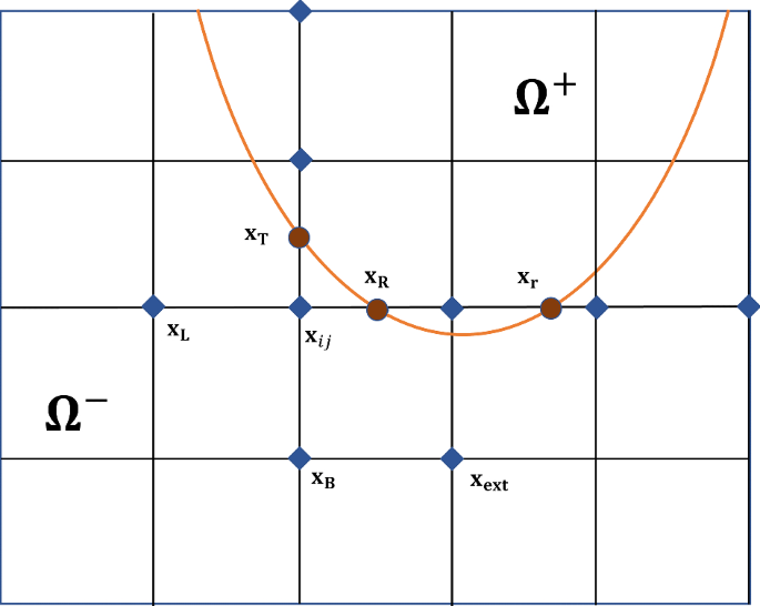

  

  Illustration for interface and points of case 3

• Case 3 The interface intersects two grid segments, but case 2 in Sect. 3.2 occurs. We again assume that ${\mathbf {x}}_{\mathbf {R}}$ and ${\mathbf {x}}_{\mathbf {T}}$ are not on the grid, but ${\mathbf {x}}_{\mathbf {B}}$ and ${\mathbf {x}}_{\mathbf {L}}$ are on the grid; however, we now have $(x_{i+2},y_{j})\in {\Omega }^-$. We define ${\mathbf {x}}_{\mathbf {r}}$ as in (31). Figure 17 shows the interface and the location of ${\mathbf {x}}_{\mathbf {r}}$. Again, quadratic interpolation (26) and second-order finite differences in Cartesian direction lead to the approximations

  $$\begin{aligned} \begin{aligned} u_x^+({\mathbf {x}}_{\mathbf {R}})&\approx \left( -\frac{3-2\theta _R -\theta _r}{(1-\theta _R)(2-\theta _R-\theta _r)} u_R^+ +\frac{2-\theta _R-\theta _r}{(1-\theta _R)(1-\theta _r)} u_{i,j}\right. \\&\quad \left. - \frac{1-\theta _R}{(1-\theta _r)(2-\theta _R-\theta _r)} u_{r}^+\right) \bigg /\varDelta x ,\\ u_x^-({\mathbf {x}}_{\mathbf {R}})&\approx \left. \left( \frac{\theta _R}{\theta _R+1} u_{i-1,j} - \frac{\theta _R+1}{\theta _R} u_{i,j}+ \frac{2\theta _R+1}{\theta _R(\theta _R+1)} u_{R}^- \right) \bigg / \varDelta x\right. ,\\ u_y^-({\mathbf {x}}_{\mathbf {R}})&\approx \left. \left( \theta _Ru_{xy}^0 + u_y^0 \right) \bigg / \varDelta y\right. \end{aligned} \end{aligned}$$

  at ${\mathbf {x}}_{\mathbf {R}}$,

  $$\begin{aligned} \begin{aligned} u_x^+({\mathbf {x}}_{\mathbf {r}})&\approx \left( \frac{ 1-\theta _r}{(1-\theta _R)(2-\theta _R-\theta _r)} u_R^+ -\frac{2-\theta _R-\theta _r}{(1-\theta _R)(1-\theta _r)} u_{i,j}\right. \\&\quad \left. + \frac{3-\theta _R-2\theta _r}{(1-\theta _r)(2-\theta _R-\theta _r)} u_{r}^+ \right) \bigg /\varDelta x ,\\ u_x^-({\mathbf {x}}_{\mathbf {r}})&\approx \left. \left( -\frac{\theta _r}{\theta _r+1} u_{i+3,j} + \frac{\theta _r+1}{\theta _r} u_{i+2,j}- \frac{2\theta _r+1}{\theta _r(\theta _r+1)} u_{r}^- \right) \bigg / \varDelta x\right. ,\\ u_y^-({\mathbf {x}}_{\mathbf {r}})&\approx \left. \left( (2-\theta _r) u_{xy}^0 + u_y^0 \right) \bigg / \varDelta y\right. \end{aligned} \end{aligned}$$

  at ${\mathbf {x}}_{\mathbf {r}}$, and

  $$\begin{aligned} \begin{aligned} u_y^+({\mathbf {x}}_{\mathbf {T}})&\approx \left. \left( -\frac{3-2\theta _T}{(1-\theta _T)(2-\theta _T)} u_T^+ +\frac{2-\theta _T}{1-\theta _T} u_{i,j+1}- \frac{1-\theta _T}{2-\theta _T} u_{i,j+2}\right) \bigg /\varDelta y \right. ,\\ u_y^-({\mathbf {x}}_{\mathbf {T}})&\approx \left. \left( \frac{\theta _T}{\theta _T+1} u_{i,j-1} - \frac{\theta _T+1}{\theta _T} u_{i,j}+ \frac{2\theta _T+1}{\theta _T(\theta _T+1)} u_{T}^- \right) \bigg / \varDelta y\right. ,\\ u_x^-({\mathbf {x}}_{\mathbf {T}})&\approx \left. \left( \theta _Tu_{xy}^0 + u_x^0 \right) \bigg / \varDelta x\right. \end{aligned} \end{aligned}$$

  at ${\mathbf {x}}_{\mathbf {T}}$ for

  $$\begin{aligned} \begin{aligned} u_{xy}^0&=\left. \left( \frac{2}{(\theta _R+1)\theta _R} u_{R} +\frac{\theta _R-2}{\theta _R} u_{i,j}-\frac{\theta _R-1}{\theta _R+1}u_{i-1,j}-u_{i+1,j-1}+u_{i,j-1} \right) \right. ,\\ u_{x}^0&=\left. \left( \frac{1}{\theta _R(\theta _R+1)}u_{R}^-+\frac{\theta _R-1}{\theta _R}u_{i,j}-\frac{\theta _R}{\theta _R+1}u_{i-1,j} \right) \right. ,\\ u_{y}^0&=\left. \left( \frac{1}{\theta _T(\theta _T+1)}u_{T}^-+\frac{\theta _T-1}{\theta _T}u_{i,j}-\frac{\theta _T}{\theta _T+1}u_{i,j-1} \right) \right. . \end{aligned} \end{aligned}$$

  By discretization of the jump conditions at ${\mathbf {x}}_{\mathbf {T}}$, ${\mathbf {x}}_{\mathbf {R}}$, and ${\mathbf {x}}_{\mathbf {r}}$, we obtain the system

  $$\begin{aligned} \mathbf {M} \begin{pmatrix} u_R^-\\ u_r^-\\ u_T^- \end{pmatrix}=\mathbf {N} \mathbf {u}+ \mathbf {d} \end{aligned}$$

  for

  $$\begin{aligned} \mathbf {M}= \left( m_{ij}\right) _{i,j=1,2,3} \end{aligned}$$

  where

  $$\begin{aligned} \begin{aligned} m_{11}&=\left( \beta ^+ \frac{(1-\theta _r)(3-2\theta _R-\theta _r)}{\hat{\theta }} +(\beta ^- +[\beta ] n_y^2) \frac{2\theta _R+1}{,}{\theta _R(\theta _R+1)}\right. \\&\quad \left. -[\beta ] n_x n_y \frac{2\theta _R}{\theta _R(\theta _R+1)} \right) \left. \right| _{\mathbf {x}={\mathbf {x}}_{\mathbf {R}}}, \\ m_{12}&=\left. \left( \beta ^+ \frac{(1-\theta _R)^2}{\hat{\theta }} \right) \right| _{\mathbf {x}={\mathbf {x}}_{\mathbf {R}}}, \\ m_{13}&=\left. \left( -[\beta ]n_x n_y\frac{1}{\theta _T(\theta _T+1)} \right) \right| _{\mathbf {x}={\mathbf {x}}_{\mathbf {R}}},\\ m_{21}&=\left. \left( \beta ^+ \frac{(1-\theta _r)^2}{\hat{\theta }} +[\beta ] n_x n_y\frac{4-2\theta _r}{\theta _R(\theta _R+1)} \right) \right| _{\mathbf {x}={\mathbf {x}}_{\mathbf {r}}},\\ m_{22}&= \left. \left( \beta ^+\frac{(3-\theta _R-2\theta _r)(1-\theta _R)}{\hat{\theta }} +(\beta ^- +[\beta ] n_y^2 )\frac{2\theta _r+1 }{\theta _r(\theta _r+1)}\right) \right| _{\mathbf {x}={\mathbf {x}}_{\mathbf {r}}},\\ m_{23}&= \left. \left( [\beta ]n_x n_y \frac{1}{\theta _T(\theta _T+1)}\right) \right| _{\mathbf {x}={\mathbf {x}}_{\mathbf {r}}},\\ m_{31}&=\left. \left( -[\beta ] n_x n_y \frac{2\theta _T+1}{\theta _R(\theta _R+1)}\right) \right| _{\mathbf {x}={\mathbf {x}}_{\mathbf {T}}},\\ m_{32}&=0,\\ m_{33}&= \left. \left( \beta ^+ \frac{3-2\theta _T}{(1-\theta _T)(2-\theta _T)} +(\beta ^- +[\beta ]n_x^2) \frac{2\theta _T+1}{\theta _T(\theta _T+1)}\right) \right| _{\mathbf {x}={\mathbf {x}}_{\mathbf {T}}} \end{aligned} \end{aligned}$$

  and

  $$\begin{aligned} \hat{\theta } = (1-\theta _r)(2-\theta _R-\theta _r)(1-\theta _R). \end{aligned}$$

  Fig. 18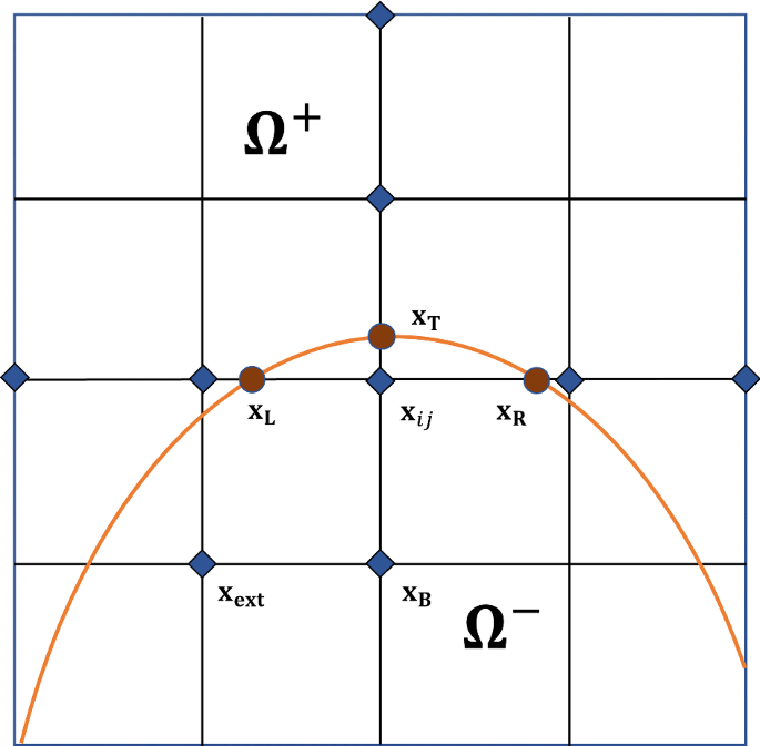

  

  Illustration for interface and points of case 4

• Case 4 The interface intersects three grid segments.

  Without loss of generality, we may assume that ${\mathbf {x}}_{\mathbf {T}},{\mathbf {x}}_{\mathbf {L}},{\mathbf {x}}_{\mathbf {R}}$ are not on the grid, and ${\mathbf {x}}_{\mathbf {B}}=(x_{i},y_{j-1})$, as shown in Fig. 18. We choose $\mathbf {x_\text {ext}} = (x_{i-1},y_{j-1})$. By quadratic interpolation (26) and second-order finite differences, at ${\mathbf {x}}_{\mathbf {R}}$, we have

  $$\begin{aligned} \begin{aligned} u_x^+({\mathbf {x}}_{\mathbf {R}})&\approx \left. \left( - \frac{1-\theta _R}{2-\theta _R} u_{i+2,j}^+ +\frac{2-\theta _R}{1-\theta _R} u_{i+1,j} -\frac{3-2\theta _R }{(1-\theta _R)(1-\theta _R)} u_R^+\right) \bigg /\varDelta x \right. ,\\ u_x^-({\mathbf {x}}_{\mathbf {R}})&\approx \left. \left( \frac{2\theta _R+\theta _L}{\theta _R(\theta _R+\theta _L)} u_{R}^- - \frac{\theta _R+\theta _L}{\theta _R\theta _L} u_{i,j}+\frac{\theta _R}{(\theta _R+\theta _L)\theta _L} u_{L}^- \right) \bigg / \varDelta x\right. ,\\ u_y^-({\mathbf {x}}_{\mathbf {R}})&\approx \left. \left( \theta _Ru_{xy}^0 + u_y^0 \right) \bigg / \varDelta y\right. . \end{aligned} \end{aligned}$$

  At ${\mathbf {x}}_{\mathbf {L}}$, we have

  $$\begin{aligned} \begin{aligned} u_x^+({\mathbf {x}}_{\mathbf {L}})&\approx \left. \left( \frac{3-2\theta _L }{(1-\theta _L)(1-\theta _L)} u_L^+ -\frac{2-\theta _L}{1-\theta _L} u_{i-1,j} + \frac{1-\theta _L}{2-\theta _L} u_{i-2,j}\right) \bigg /\varDelta x \right. ,\\ u_x^-({\mathbf {x}}_{\mathbf {L}})&\approx \left. \left( -\frac{\theta _L}{\theta _R(\theta _R+\theta _L)} u_{R}^- +\frac{\theta _R+\theta _L}{\theta _R\theta _L} u_{i,j}-\frac{\theta _R+2\theta _L}{(\theta _R+\theta _L)\theta _L} u_{L}^- \right) \bigg / \varDelta x\right. ,\\ u_y^-({\mathbf {x}}_{\mathbf {L}})&\approx \left. \left( -\theta _Lu_{xy}^0 + u_y^0 \right) \bigg / \varDelta y\right. \end{aligned} \end{aligned}$$

  and at ${\mathbf {x}}_{\mathbf {T}}$, we have

  $$\begin{aligned} \begin{aligned} u_y^+({\mathbf {x}}_{\mathbf {T}})&\approx \left. \left( -\frac{3-2\theta _T}{(1-\theta _T)(2-\theta _T)} u_T^+ +\frac{2-\theta _T}{1-\theta _T} u_{i,j+1}- \frac{1-\theta _T}{2-\theta _T} u_{i,j+2}\right) \bigg /\varDelta y \right. ,\\ u_y^-({\mathbf {x}}_{\mathbf {T}})&\approx \left. \left( \frac{\theta _T}{\theta _T+1} u_{i,j-1} - \frac{\theta _T+1}{\theta _T} u_{i,j}+ \frac{2\theta _T+1}{\theta _T(\theta _T+1)} u_{T}^- \right) \bigg / \varDelta y\right. ,\\ u_x^-({\mathbf {x}}_{\mathbf {T}})&\approx \left. \left( \theta _Tu_{xy}^0 + u_x^0 \right) \bigg / \varDelta x\right. \end{aligned} \end{aligned}$$

  for

  $$\begin{aligned} \begin{aligned} u_{xy}^0&=\left. \left( \frac{\theta _L-1}{(\theta _R+\theta _L)\theta _R} u_{R}^- {+}\frac{\theta _R-\theta _L+1}{\theta _R\theta _L} u_{i,j}{-}\frac{\theta _R+1}{(\theta _R+\theta _L)\theta _L}u_{L}{-}u_{i,j-1}{+}u_{i-1,j-1} \right) \right. ,\\ u_{x}^0&=\left. \left( \frac{\theta _L}{\theta _R(\theta _R+\theta _L)}u_{R}^-+\frac{\theta _R-\theta _L}{\theta _R\theta _L}u_{i,j}-\frac{\theta _R}{(\theta _R+\theta _L)\theta _L}u_{L}^- \right) \right. ,\\ u_{y}^0&=\left. \left( \frac{1}{\theta _T(\theta _T+1)}u_{T}^-+\frac{\theta _T-1}{\theta _T}u_{i,j}-\frac{\theta _T}{\theta _T+1}u_{i,j-1} \right) \right. . \end{aligned} \end{aligned}$$

  We discretize the jump conditions

  $$\begin{aligned}{}[\beta u_n]n_x -[\beta ](-u_x^- n_y + u_y^-n_x)n_y -\beta ^+[u]_\tau n_y = \beta ^+u_x^+ - \beta ^- u_x^- \end{aligned}$$

  at ${\mathbf {x}}_{\mathbf {L}},{\mathbf {x}}_{\mathbf {R}}$, and

  $$\begin{aligned} \begin{aligned}{}[\beta u_n]n_y +[\beta ](-u_x^- n_y + u_y^-n_x)n_x +\beta ^+[u]_\tau n_x = \beta ^+u_y^+ - \beta ^- u_y^- \end{aligned} \end{aligned}$$

  at ${\mathbf {x}}_{\mathbf {T}}$ to obtain

  $$\begin{aligned} \mathbf {M} \begin{pmatrix} u_L^-\\ u_R^-\\ u_T^- \end{pmatrix}=\mathbf {N} \mathbf {u}+ \mathbf {d} \end{aligned}$$

  for

  $$\begin{aligned} \mathbf {M}= \left( m_{ij}\right) _{i,j=1,2,3} \end{aligned}$$

  where

  $$\begin{aligned} m_{11}&=\left. \left( \beta ^+ \frac{3-2\theta _L}{(1-\theta _L)(2-\theta _L)} +(\beta ^- + [\beta ] n_y^2) \frac{2\theta _L\theta _R+\theta _R^2}{\hat{\theta }}+ [\beta ] n_y n_x \frac{(\theta _R+\theta _R^2)\theta _L}{\hat{\theta }}\right) \right| _{\mathbf {x}={\mathbf {x}}_{\mathbf {L}}} ,\\ m_{12}&=\left. \left( \beta ^-+ [\beta ] n_y^2 \frac{(\theta _L)^2}{\hat{\theta }}+ [\beta ] n_x n_y \frac{-(\theta _L)^3+(\theta _L)^2}{\hat{\theta }}\right) \right| _{\mathbf {x}={\mathbf {x}}_{\mathbf {L}}},\\ m_{13}&=\left. \left( [\beta ]n_y n_x \frac{1}{\theta _T(\theta _T+1)}\right) \right| _{\mathbf {x}={\mathbf {x}}_{\mathbf {L}}},\\ m_{21}&=\left. \left( \beta ^-+ [\beta ] n_y^2 \frac{(\theta _R)^2}{\hat{\theta }}+ [\beta ] n_x n_y \frac{(\theta _R)^3+(\theta _R)^2}{\hat{\theta }}\right) \right| _{\mathbf {x}={\mathbf {x}}_{\mathbf {R}}}, \\ m_{22}&=\left. \left( \beta ^+ \frac{3-2\theta _R}{(1-\theta _R)(2-\theta _R)} +(\beta ^- + [\beta ] n_y^2 )\frac{2\theta _L\theta _R+(\theta _L)^2}{\hat{\theta }}+ [\beta ] n_y n_x \frac{(\theta _L-(\theta _L)^2)\theta _R}{\hat{\theta }}\right) \right| _{\mathbf {x}={\mathbf {x}}_{\mathbf {R}}}, \\ m_{23}&= \left. \left( -[\beta ]n_y n_x \frac{1}{\theta _T(\theta _T+1)}\right) \right| _{\mathbf {x}={\mathbf {x}}_{\mathbf {R}}},\\ m_{31}&=\left. \left( -[\beta ] n_x n_y \frac{(\theta _R)^2 +(\theta _R+(\theta _R)^2)\theta _T}{\hat{\theta }}\right) \right| _{\mathbf {x}={\mathbf {x}}_{\mathbf {T}}},\\ m_{32}&=\left. \left( [\beta ] n_x n_y \frac{(\theta _L)^2 +(-\theta _L+(\theta _L)^2)\theta _T}{\hat{\theta }}\right) \right| _{\mathbf {x}={\mathbf {x}}_{\mathbf {T}}},\\ m_{33}&=\left. \left( \beta ^+ \frac{3-2\theta _T}{(1-\theta _T)(2-\theta _T)} +(\beta ^- + [\beta ] n_x^2) \frac{2\theta _T+1}{\theta _T(\theta _T+1)}\right) \right| _{\mathbf {x}={\mathbf {x}}_{\mathbf {T}}} \end{aligned}$$

  and

  $$\begin{aligned} \hat{\theta } = \theta _R(\theta _R+\theta _L)\theta _L. \end{aligned}$$

References

Chen, X., Feng, X., Li, Z.: A direct method for accurate solution and gradient computations for elliptic interface problems. Numer. Algorithms 80(3), 709–740 (2019)
Chern, I.L., Shu, Y.C.: A coupling interface method for elliptic interface problems. J. Comput. Phys. 225(2), 2138–2174 (2007)
Coco, A., Russo, G.: Second order finite-difference ghost-point multigrid methods for elliptic problems with discontinuous coefficients on an arbitrary interface. J. Comput. Phys. 361, 299–330 (2018)
Gibou, F., Fedkiw, R.P., Cheng, L.T., Kang, M.: A second-order-accurate symmetric discretization of the Poisson equation on irregular domains. J. Comput. Phys. 176(1), 205–227 (2002)
Guittet, A., Lepilliez, M., Tanguy, S., Gibou, F.: Solving elliptic problems with discontinuities on irregular domains-the Voronoi interface method. J. Comput. Phys. 298, 747–765 (2015)
Lee, L., LeVeque, R.J.: An immersed interface method for incompressible Navier–Stokes equations. SIAM J. Sci. Comput. 25(3), 832–856 (2003)
Leveque, R.J., Li, Z.: The immersed interface method for elliptic equations with discontinuous coefficients and singular sources. SIAM J. Numer. Anal. 31(4), 1019–1044 (1994)
LeVeque, R.J., Li, Z.: Immersed interface methods for Stokes flow with elastic boundaries or surface tension. SIAM J. Sci. Comput. 18(3), 709–735 (1997)
Li, Z.: A fast iterative algorithm for elliptic interface problems. SIAM J. Numer. Anal. 35(1), 230–254 (1998)
Li, Z., Lai, M.C.: The immersed interface method for the Navier–Stokes equations with singular forces. J. Comput. Phys. 171(2), 822–842 (2001)
Li, Z., Ji, H., Chen, X.: Accurate solution and gradient computation for elliptic interface problems with variable coefficients. SIAM J. Numer. Anal. 55(2), 570–597 (2017). https://doi.org/10.1137/15M1040244
Linnick, M.N., Fasel, H.F.: A high-order immersed interface method for simulating unsteady incompressible flows on irregular domains. J. Comput. Phys. 204(1), 157–192 (2005)
Liu, X.D., Fedkiw, R.P., Kang, M.: A boundary condition capturing method for Poisson’s equation on irregular domains. J. Comput. Phys. 160(1), 151–178 (2000)
Marques, A.N., Nave, J.C., Rosales, R.R.: A correction function method for Poisson problems with interface jump conditions. J. Comput. Phys. 230(20), 7567–7597 (2011)
Marques, A.N., Nave, J.C., Rosales, R.R.: High order solution of Poisson problems with piecewise constant coefficients and interface jumps. J. Comput. Phys. 335, 497–515 (2017)
Osher, S., Sethian, J.A.: Fronts propagating with curvature-dependent speed: algorithms based on Hamilton–Jacobi formulations. J. Comput. Phys. 79(1), 12–49 (1988)
Saad, Y.: Iterative Methods for Sparse Linear Systems, vol. 82. SIAM, Philadelphia (2003)
Seo, J., Ha, Sy, Min, C.: Convergence analysis in the maximum norm of the numerical gradient of the Shortley–Weller method. J. Sci. Comput. 74(2), 631–639 (2018)
Shortley, G.H., Weller, R.: The numerical solution of Laplace’s equation. J. Appl. Phys. 9(5), 334–348 (1938)
Wiegmann, A., Bube, K.P.: The explicit-jump immersed interface method: finite difference methods for PDEs with piecewise smooth solutions. SIAM J. Numer. Anal. 37(3), 827–862 (2000)
Yoon, G., Min, C.: A review of the supra-convergences of Shortley–Weller method for Poisson equation. J. KSIAM 18(1), 51–60 (2014)
Yoon, G., Min, C.: Analyses on the finite difference method by Gibou et al. for Poisson equation. J. Comput. Phys. 280, 184–194 (2015)
Acknowledgements
The research of Byungjoon Lee was supported by NRF Grant 2017R1C1B1008626 and POSCO Science Fellowship of POSCO TJ Park Foundation. The research of Myungjoo Kang was supported by the National Research Foundation of Korea (NRF)(2015R1A15A1009350, 2017R1A2A1A17069644).
Author information
Authors and Affiliations
Corresponding author
Additional information
Publisher's Note
Springer Nature remains neutral with regard to jurisdictional claims in published maps and institutional affiliations.