Reliable networking in Ethernet ring mesh networks using regular topologies

Abstract

Reliable networking is an important factor in Ethernet ring mesh networks (ERMs) with ITU-T G.8032 Ethernet ring protection recommendation or with the IEC 62439-3 high-availability seamless redundancy protocol. However, there are two major challenges for this purpose: (1) Hitherto, irregular topologies are used in ERMs that it causes difficulty in analyzing and improving reliability. (2) A topology is appropriate for practical implementation, if it is low cost, simple to implement, and simple to develop for large scale-systems (i.e. scalable). However, irregular topologies are extremely difficult to implement and develop. To deal with these challenges, this paper introduces two regular topologies called chordal ring and k-cube networks, for the first time in the area of ERMs. In addition, the proposed topologies are carefully analyzed in terms of reliability. These analyzes prove that the proposed regular topologies outperform existing irregular multiple-ring networks namely shared link, shared node, complex shared link, redundant link, and 3-connected network.

Appendix

Here, how to use the decomposition method (DM) for calculating the all-terminal reliability equations in Sect. 4.1 will be described in detail.

• (1) Shared link topology reliability (Eq. 4): First, we examine Eq. (4), which is related to the reliability of shared link topology. How to choose DM key components is shown appropriately by a hierarchical graph in Fig. 6. In this figure, the key components are labeled by $k_{1}$, $k_{2}$, $k_{3}$, and $k_{4}$, in the order they were selected. Two states corresponding to each key component (healthy or failed) is also shown in Fig. 6. For example, $\overline{{k_{1} }}$ is indicative of the failure of first key component.

  Fig. 6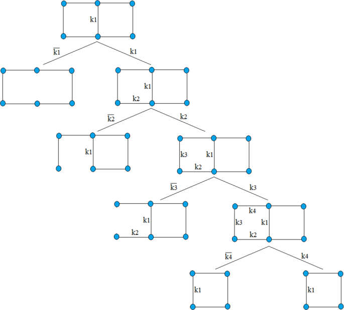

  

  The hierarchy of the key components in the decomposition method for shared link topology

Using Fig. 6, we can calculate the network reliability related to different network states according to different states of key components that are shown by a sequence of key components and their states:

$$ \overline{{k_{1} }} = 6e^{ - 5\lambda t} - 5e^{ - 6\lambda t} $$

(33)

$$ k_{1} \overline{{k_{2} }} = e^{ - 2\lambda t} \left( {3e^{ - 2\lambda t} - 2e^{ - 3\lambda t} } \right) $$

(34)

$$ k_{1} k_{2} \overline{{k_{3} }} = e^{ - \lambda t} \left( {3e^{ - 2\lambda t} - 2e^{ - 3\lambda t} } \right) $$

(35)

$$ k_{1} k_{2} k_{3} \overline{{k_{4} }} = 3e^{ - 2\lambda t} - 2e^{ - 3\lambda t} $$

(36)

$$ k_{1} k_{2} k_{3} k_{4} = 3e^{ - 2\lambda t} - 2e^{ - 3\lambda t} $$

(37)

Now, according to Eqs. (33)–(37), the reliability of the entire network can be calculated as follows (i.e. equal to the Eq. (4) in the previous section):

$$ \begin{aligned} R_{shared link} \left( t \right) & = \left( {1 - e^{ - \lambda t} } \right)\left( {6e^{ - 5\lambda t} - 5e^{ - 6\lambda t} } \right) \\ & \quad + {\kern 1pt} e^{ - \lambda t} \left( {e^{ - 2\lambda t} \left( {3e^{ - 2\lambda t} - 2e^{ - 3\lambda t} } \right)\left( {1 - e^{ - \lambda t} } \right)} \right. \\ & \quad + {\kern 1pt} e^{ - \lambda t} \left( {e^{ - \lambda t} \left( {3e^{ - 2\lambda t} - 2e^{ - 3\lambda t} } \right)\left( {1 - e^{ - \lambda t} } \right)} \right. \\ & \quad + {\kern 1pt} e^{ - \lambda t} \left. \left. \left( \left( {3e^{ - 2\lambda t} - 2e^{ - 3\lambda t} } \right)\left( {1 - e^{ - \lambda t} } \right) \right.\right.\right.\\ &\quad + e^{ - \lambda t}\left. \left.\left. \left( {3e^{ - 2\lambda t} - 2e^{ - 3\lambda t} } \right) \right) \right) \right) \\ & = 15e^{ - 5\lambda t} - 23e^{ - 6\lambda t} + 9e^{ - 7\lambda t} \\ \end{aligned} $$

(38)

• (2) Shared node topology (Eq. 5): The hierarchy diagram of the key components selection for shared node topology is shown in Fig. 7. Considering this figure, we have:

  Fig. 7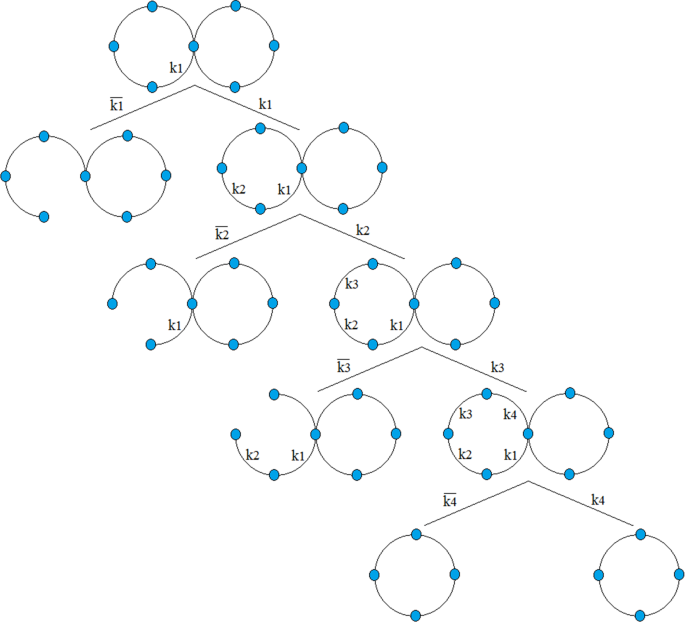

  

  The hierarchy of the key components in the decomposition method for shared node topology

  $$ \overline{{k_{1} }} = e^{ - 3\lambda t} \left( {4e^{ - 3\lambda t} - 3e^{ - 4\lambda t} } \right) $$

  (39)
  $$ k_{1} \overline{{k_{2} }} = e^{ - 2\lambda t} \left( {4e^{ - 3\lambda t} - 3e^{ - 4\lambda t} } \right) $$

  (40)
  $$ k_{1} k_{2} \overline{{k_{3} }} = e^{ - \lambda t} \left( {4e^{ - 3\lambda t} - 3e^{ - 4\lambda t} } \right) $$

  (41)
  $$ k_{1} k_{2} k_{3} \overline{{k_{4} }} = 4e^{ - 3\lambda t} - 3e^{ - 4\lambda t} $$

  (42)
  $$ k_{1} k_{2} k_{3} k_{4} = 4e^{ - 3\lambda t} - 3e^{ - 4\lambda t} $$

  (43)

As a result, according to Eqs. (39)–(43), the reliability of the entire network is given by (i.e. equal to the Eq. 5):

$$ \begin{aligned} R_{shared node} \left( t \right) & = \left( {1 - e^{ - \lambda t} } \right)\left( {e^{ - 3\lambda t} \left( {4e^{ - 3\lambda t} - 3e^{ - 4\lambda t} } \right)} \right) \\ & \quad + {\kern 1pt} e^{ - \lambda t} \left( {e^{ - 2\lambda t} \left( {4e^{ - 3\lambda t} - 3e^{ - 4\lambda t} } \right)\left( {1 - e^{ - \lambda t} } \right)} \right. \\ & \quad + {\kern 1pt} e^{ - \lambda t} \left( {e^{ - \lambda t} \left( {4e^{ - 3\lambda t} - 3e^{ - 4\lambda t} } \right)\left( {1 - e^{ - \lambda t} } \right)} \right. \\ & \quad + {\kern 1pt} e^{ - \lambda t} \left. \left. \left( \left( {4e^{ - 3\lambda t} - 3e^{ - 4\lambda t} } \right)\left( {1 - e^{ - \lambda t} } \right) \right.\right.\right.\\ &\quad + e^{ - \lambda t} \left.\left.\left. \left( {4e^{ - 3\lambda t} - 3e^{ - 4\lambda t} } \right) \right) \right) \right) \\ & = 16e^{ - 6\lambda t} - 24e^{ - 7\lambda t} + 9e^{ - 8\lambda t} \\ \end{aligned} $$

(44)

• (3) Complex shared link topology (Eq. 6): The hierarchy diagram of the key components selection for complex shared link topology is shown in Fig. 8. Considering this figure, network reliability for different modes is as follows:

  Fig. 8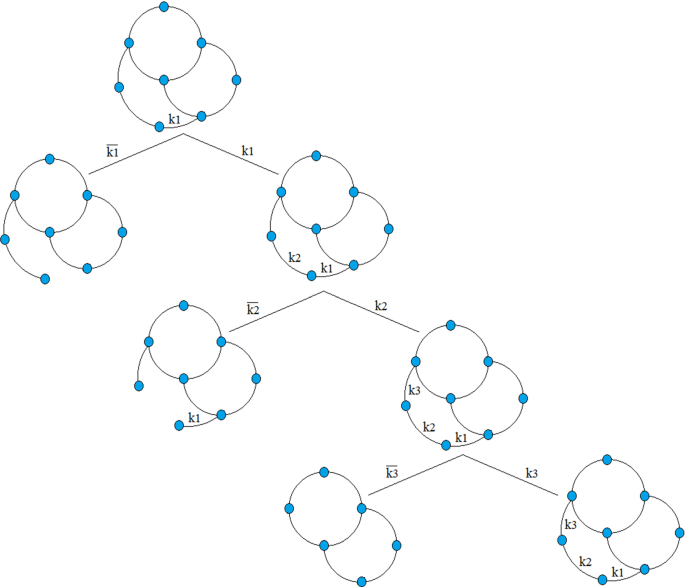

  

  The hierarchy of the key components in the decomposition method for complex shared link topology

  $$ \overline{{k_{1} }} = e^{ - 2\lambda t} \left( {15e^{ - 5\lambda t} - 23e^{ - 6\lambda t} + 9e^{ - 7\lambda t} } \right) $$

  (45)
  $$ k_{1} \overline{{k_{2} }} = e^{ - \lambda t} \left( {15e^{ - 5\lambda t} - 23e^{ - 6\lambda t} + 9e^{ - 7\lambda t} } \right) $$

  (46)
  $$ k_{1} k_{2} \overline{{k_{3} }} = 15e^{ - 5\lambda t} - 23e^{ - 6\lambda t} + 9e^{ - 7\lambda t} $$

  (47)
  $$ \begin{aligned} k_{1} k_{2} k_{3} & = \left( {1 - e^{ - \lambda t} } \right)\left( {e^{ - \lambda t} \left( {1 - e^{ - \lambda t} } \right)\left( {4e^{ - 3\lambda t} - 3e^{ - 4\lambda t} } \right)} \right. \\ & \quad \left. +\, {\kern 1pt} e^{ - \lambda t} \left( \left( {1 - e^{ - \lambda t} } \right)\left( {4e^{ - 3\lambda t} - 3e^{ - 4\lambda t} } \right) \right.\right.\\ &\quad + e^{ - \lambda t}\left.\left. \left( {4e^{ - 2\lambda t} - 4e^{ - 3\lambda t} + e^{ - 4\lambda t} } \right) \right) \right) \\ & \quad + {\kern 1pt} e^{ - \lambda t} \left( \left( {1 - e^{ - \lambda t} } \right)\left( {4e^{ - 3\lambda t} - 3e^{ - 4\lambda t} } \right) \right. \\ &\quad + e^{ - \lambda t} \left. \left( {4e^{ - 2\lambda t} - 4e^{ - 3\lambda t} + e^{ - 4\lambda t} } \right) \right) \\ & = 20e^{ - 4\lambda t} - 41e^{ - 5\lambda t} + 29e^{ - 6\lambda t} - 7e^{ - 7\lambda t} \\ \end{aligned} $$

  (48)

Therefore, according to the Eqs. (45)–(48), we have:

$$ \begin{aligned} & R_{complex shared link} \left( t \right) \\ & \quad = \left( {1 - e^{ - \lambda t} } \right)\left( {e^{ - 2\lambda t} \left( {15e^{ - 5\lambda t} - 23e^{ - 6\lambda t} + 9e^{ - 7\lambda t} } \right)} \right) \\ & \qquad + {\kern 1pt} e^{ - \lambda t} \left( {\left( {15e^{ - 5\lambda t} - 23e^{ - 6\lambda t} + 9e^{ - 7\lambda t} } \right)\left( {1 - e^{ - \lambda t} } \right)} \right. \\ & \qquad + {\kern 1pt} e^{ - \lambda t} \left( {\left( {15e^{ - 5\lambda t} - 23e^{ - 6\lambda t} + 9e^{ - 7\lambda t} } \right)\left( {1 - e^{ - \lambda t} } \right)} \right. \\ & \qquad + {\kern 1pt} e^{ - \lambda t} \left( {\left( {1 - e^{ - \lambda t} } \right)\left( {e^{ - \lambda t} \left( {1 - e^{ - \lambda t} } \right)\left( {4e^{ - 3\lambda t} - 3e^{ - 4\lambda t} } \right)} \right.} \right. \\ & \qquad + {\kern 1pt} e^{ - \lambda t} \left( \left( {1 - e^{ - \lambda t} } \right)\left( {4e^{ - 3\lambda t} - 3e^{ - 4\lambda t} } \right) \right. \\ &\qquad +\, e^{ - \lambda t} \left. \left. {\left. {\left( {4e^{ - 2\lambda t} - 4e^{ - 3\lambda t} + e^{ - 4\lambda t} } \right)} \right)} \right) \right. \\ & \qquad +\, {\kern 1pt} e^{ - \lambda t} \left( \left( {1 - e^{ - \lambda t} } \right)\left( {4e^{ - 3\lambda t} - 3e^{ - 4\lambda t} } \right) \right.\\ &\qquad + e^{ - \lambda t} \left. \right.\left. {\left. {\left. {\left. {\left( {4e^{ - 2\lambda t} - 4e^{ - 3\lambda t} + e^{ - 4\lambda t} } \right)} \right)} \right)} \right)} \right) \\ & \quad = 65e^{ - 7\lambda t} - 155e^{ - 8\lambda t} + 125e^{ - 9\lambda t} - 34e^{ - 10\lambda t} \\ \end{aligned} $$

(49)

• (4) Redundant link topology (Eq. 7): Based on the hierarchy of the key components selection for redundant topology that is shown in Fig. 9, network reliability related to different network states according to different states of key components are given by:

  Fig. 9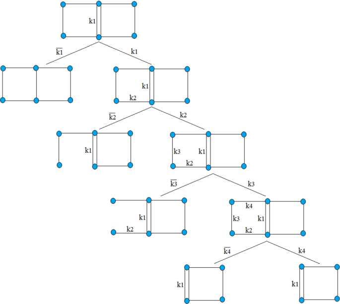

  

  The hierarchy of the key components in the decomposition method for redundant link topology

  $$ \overline{{k_{1} }} = 15e^{ - 5\lambda t} - 23e^{ - 6\lambda t} + 9e^{ - 7\lambda t} $$

  (50)
  $$ k_{1} \overline{{k_{2} }} = e^{ - 2\lambda t} \left( {3e^{ - 2\lambda t} - 2e^{ - 3\lambda t} } \right) $$

  (51)
  $$ k_{1} k_{2} \overline{{k_{3} }} = e^{ - \lambda t} \left( {3e^{ - 2\lambda t} - 2e^{ - 3\lambda t} } \right) $$

  (52)
  $$ k_{1} k_{2} k_{3} \overline{{k_{4} }} = 3e^{ - 2\lambda t} - 2e^{ - 3\lambda t} $$

  (53)
  $$ k_{1} k_{2} k_{3} k_{4} = 3e^{ - 2\lambda t} - 2e^{ - 3\lambda t} $$

  (54)

According to the above equations, the reliability of the entire network is calculated as follows:

$$ \begin{aligned} & R_{redundant link} \left( t \right) \\ & \quad = \left( {1 - e^{ - \lambda t} } \right)\left( {15e^{ - 5\lambda t} - 23e^{ - 6\lambda t} + 9e^{ - 7\lambda t} } \right) \\ & \quad\quad\quad + e^{ - \lambda t} \left( {e^{ - 2\lambda t} \left( {3e^{ - 2\lambda t} - 2e^{ - 3\lambda t} } \right)\left( {1 - e^{ - \lambda t} } \right)} \right. \\ & \quad\quad\quad + e^{ - \lambda t} \left( {e^{ - \lambda t} \left( {3e^{ - 2\lambda t} - 2e^{ - 3\lambda t} } \right)\left( {1 - e^{ - \lambda t} } \right)} \right. \\ & \left. \left. \quad\quad\quad +\, e^{ - \lambda t} \left( \left( {3e^{ - 2\lambda t} - 2e^{ - 3\lambda t} } \right)\left( {1 - e^{ - \lambda t} } \right) \right.\right.\right.\\ &\quad\quad\quad \left.\left.\left. +\, e^{ - \lambda t} \left( {3e^{ - 2\lambda t} - 2e^{ - 3\lambda t} } \right) \right) \right) \right) \\ & \quad = 24e^{ - 5\lambda t} - 50e^{ - 6\lambda t} + 36e^{ - 7\lambda t} - 9e^{ - 8\lambda t} \\ \end{aligned} $$

(55)

• (5) 3-Connected network (Eq. 8): How to choose key components in decomposition method for the 3-connected network is shown in Fig. 10. Based on this figure, network reliability for different modes of key components is given by:

  Fig. 10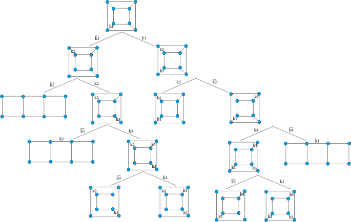

  

  The hierarchy of the key components in the decomposition method for 3-connected network

  $$ \overline{{k_{1} }} \overline{{k_{2} }} = E_{1} = 56e^{ - 7\lambda t} - 130e^{ - 8\lambda t} + 102e^{ - 9\lambda t} - 27e^{ - 10\lambda t} $$

  (56)
  $$ \overline{{k_{1} }} k_{2} \overline{{k_{3} }} = E_{2} = 40e^{ - 6\lambda t} - 90e^{ - 7\lambda t} + 69e^{ - 8\lambda t} - 18e^{ - 9\lambda t} $$

  (57)
  $$ \overline{{k_{1} }} k_{2} k_{3} \overline{{k_{4} }} = E_{3} = 32e^{ - 5\lambda t} - 68e^{ - 6\lambda t} + 49e^{ - 7\lambda t} - 12e^{ - 8\lambda t} $$

  (58)
  $$ \begin{aligned} \overline{{k_{1} }} k_{2} k_{3} k_{4} & = E_{4} = 32e^{ - 4\lambda t} - 84e^{ - 5\lambda t} \\ &\quad + 86e^{ - 6\lambda t} - 40e^{ - 7\lambda t} + 7e^{ - 8\lambda t} \end{aligned} $$

  (59)
  $$ k_{1} \overline{{k_{2} }} \overline{{k_{4} }} = E_{2} = 40e^{ - 6\lambda t} - 90e^{ - 7\lambda t} + 69e^{ - 8\lambda t} - 18e^{ - 9\lambda t} $$

  (60)
  $$ k_{1} \overline{{k_{2} }} k_{4} \overline{{k_{3} }} = E_{3} = 32e^{ - 5\lambda t} - 68e^{ - 6\lambda t} + 49e^{ - 7\lambda t} - 12e^{ - 8\lambda t} $$

  (61)
  $$\begin{aligned} k_{1} \overline{{k_{2} }} k_{4} k_{3} & = E_{4} = 32e^{ - 4\lambda t} - 84e^{ - 5\lambda t} \\ &\quad + 86e^{ - 6\lambda t} - 40e^{ - 7\lambda t} + 7e^{ - 8\lambda t} \end{aligned} $$

  (62)
  $$\begin{aligned} k_{1} k_{2} & = E_{5} = 112e^{ - 5\lambda t} - 398e^{ - 6\lambda t} + 582e^{ - 7\lambda t} \\ &\quad - 434e^{ - 8\lambda t} + 164e^{ - 9\lambda t} - 25e^{ - 10\lambda t} \end{aligned} $$

  (63)

Considering the Eqs. (56)–(63), the reliability of the 3-connected network is calculated as Eq. (64):

$$ \begin{aligned} & R_{3 - connected} \left( t \right) \\ & \quad = \left( {1 - e^{ - \lambda t} } \right)\left( \left( {1 - e^{ - \lambda t} } \right)\left( {E_{1} } \right) +\, e^{ - \lambda t} \left( \left( {1 - e^{ - \lambda t} } \right)\left( {E_{2} } \right) \right.\right.\\ &\qquad + e^{ - \lambda t} \left.\left. \left( {\left( {1 - e^{ - \lambda t} } \right)\left( {E_{3} } \right) + e^{ - \lambda t} \left( {E_{4} } \right)} \right) \right) \right) \\ & \qquad + e^{ - \lambda t} \left( \left( {1 - e^{ - \lambda t} } \right)\left( \left( {1 - e^{ - \lambda t} } \right)\left( {E_{2} } \right) \right.\right.\\ &\qquad + e^{ - \lambda t} \left.\left.\left( {\left( {1 - e^{ - \lambda t} } \right)\left( {E_{3} } \right) + e^{ - \lambda t} \left( {E_{4} } \right)} \right) \right) +\, e^{ - \lambda t} \left( {E_{5} } \right) \right) \\ & \quad = 376e^{ - 7\lambda t} - 1476e^{ - 8\lambda t} + 2352e^{ - 9\lambda t} \\ &\qquad - 1895e^{ - 10\lambda t} + 770e^{ - 11\lambda t} - 126e^{ - 12\lambda t} \\ \end{aligned} $$

(64)

• (6) Chordal rings (Eqs. (25)–(28)): To calculate the reliability of the chordal rings of $CHR4\left( {8; 2} \right)$ and $CHR4\left( {16; 2} \right)$, two cases have been considered: When all the chord links have failed (lower bound) and when all the chord links are active and healthy (upper bound). In case of lower bound for a $CHR4\left( {p; q} \right)$, network reliability is the reliability of a $p$-node single-ring network. Reliability block diagram (RBD) related to the lower bound is shown in Fig. 11(a). In addition, in the event of upper bound for a $CHR4\left( {p; q} \right)$, network reliability is equal to the reliability of a parallel system contains $p$ components in parallel from the standpoint of reliability. Figure 11(b) shows the RBD related to this case.

  Fig. 11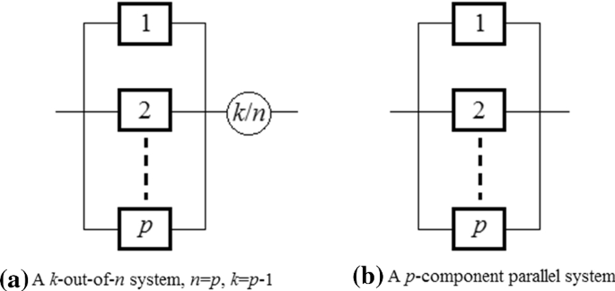

  

  a Lower bound RBD of $CHR4\left( {p; q} \right)$, b upper bound RBD of $CHR4\left( {p; q} \right)$

Therefore, according to Fig. 11a, the lower bound reliability for $CHR4\left( {8; 2} \right)$ and $CHR4\left( {16; 2} \right)$ is given by:

$$ R_{{CHR4\left( {8; 2} \right)}} \left( t \right) = 8e^{ - 7\lambda t} - 7e^{ - 8\lambda t} $$

(65)

$$ R_{{CHR4\left( {16; 2} \right)}} \left( t \right) = 16e^{ - 15\lambda t} - 15e^{ - 16\lambda t} $$

(66)

Also, according to Fig. 11b, the upper bound reliability of $CHR4\left( {8; 2} \right)$ and $CHR4\left( {16; 2} \right)$ is calculated as follows:

$$ \begin{aligned} & R_{{CHR4\left( {8; 2} \right)}} \left( t \right) \\ & \quad = 1 - \left( {1 - e^{ - \lambda t} } \right)^{8} \\ & \quad = 8e^{ - \lambda t} - 28e^{ - 2\lambda t} + 56e^{ - 3\lambda t} - 70e^{ - 4\lambda t} \\ & \qquad + 56e^{ - 5\lambda t} - 28e^{ - 6\lambda t} + 8e^{ - 7\lambda t} - e^{ - 8\lambda t} \\ \end{aligned} $$

(67)

$$ \begin{aligned} & R_{{CHR4\left( {16; 2} \right)}} \left( t \right) = 1 - \left( {1 - e^{ - \lambda t} } \right)^{16} \\ & \quad = {\kern 1pt} 16e^{ - \lambda t} - 120e^{ - 2\lambda t} + 560e^{ - 3\lambda t} - 1820e^{ - 4\lambda t}\\ & \qquad + 4368e^{ - 5\lambda t} - 8008e^{ - 6\lambda t} \\ & \qquad + {\kern 1pt} 11440e^{ - 7\lambda t} - 12870e^{ - 8\lambda t} + 11440e^{ - 9\lambda t} \\ & \qquad - 8008e^{ - 10\lambda t} + 4368e^{ - 11\lambda t} - 1820e^{ - 12\lambda t} \\ & \qquad + {\kern 1pt} {\kern 1pt} 560e^{ - 13\lambda t} - 120e^{ - 14\lambda t} + 16e^{ - 15\lambda t} - e^{ - 16\lambda t} \\ \end{aligned} $$

(68)

• (7) k-cube networks (Eqs. 25–28): 3-cube network structure is topologically equivalent to the structure of a 3-connected network. Therefore, the reliability of the 3-cube is equal to 3-connected reliability. In case of 4-cube, two modes are intended for calculation of reliability: When all the links between the two 3-cubes are failed, except for one of the links because working at least one of them is necessary for working the entire network (lower bound). In this case, reliability of the network is equal to the reliability of two 3-connected networks that are connected in series. Second mode, when all the links between the two 3-cubes are active and healthy (upper bound). In this case, the network can be seen as a 3-cube network with redundant links.

Therefore, according to the above description, the 3-cube reliability can be calculated as follows:

$$ \begin{aligned} R_{3 - cube} \left( t \right) & = 376e^{ - 7\lambda t} - 1476e^{ - 8\lambda t} + 2352e^{ - 9\lambda t} \\ & \quad - 1895e^{ - 10\lambda t} + 770e^{ - 11\lambda t} - 126e^{ - 12\lambda t} \\ \end{aligned} $$

(69)

Also, according to the above description, the 4-cube lower bound reliability is given by:

$$ R_{4 - cube} \left( t \right) = \left( {R_{3 - cube} \left( t \right)} \right)\left( {R_{3 - cube} \left( t \right)} \right) $$

(70)

Moreover, the 4-cube upper bound reliability can be defined as the a 3-cube network reliability with the difference that its link failure rate ($\lambda_{p}$) is equal to the failure rate of a parallel system includes two 3-cube links with failure rate $\lambda$:

$$ \begin{aligned} R_{4 - cube} \left( t \right) & = 376e^{{ - 7\lambda_{p} t}} - 1476e^{{ - 8\lambda_{p} t}} + 2352e^{{ - 9\lambda_{p} t}} \\ & \quad - 1895e^{{ - 10\lambda_{p} t}} + 770e^{{ - 11\lambda_{p} t}} - 126e^{{ - 12\lambda_{p} t}} \\ \end{aligned} $$

(71)

In Eq. (71), $\lambda_{p}$ is equal to:

$$ \begin{aligned} & \lambda_{p} = \frac{1}{{1 - \left( {1 - e^{ - \lambda t} } \right)^{2} }}\left( { - \frac{{d\left( {1 - \left( {1 - e^{ - \lambda t} } \right)^{2} } \right)}}{dt}} \right) \\ & \quad = \frac{{2\lambda \left( { - \frac{1}{{\varvec{e}^{t\lambda } }} + 1} \right)}}{{ - \frac{1}{{\varvec{e}^{t\lambda } }} + 2}} \\ \end{aligned} $$

(72)

References

Ryoo, J.-d., et al. (2008). Ethernet ring protection for carrier Ethernet networks. IEEE Communications Magazine, 46(9), 136–143.
Lee, D., et al. (2011). Efficient Ethernet ring mesh network design. Journal of Lightwave Technology, 29(18), 2677–2683.
Infonetics Research. (2007). Service provider plans for metro optical and Ethernet: North America, Europe, and Asia Pacific 2007, September 2007.
Allawi, Y. M., et al. (2015). Cost-effective topology design for HSR resilient mesh networks. Journal of Optical Communications and Networking, 7(1), 8–20.
Lee, K., et al. (2013). Reliable network design for Ethernet ring mesh networks. Journal of Lightwave Technology, 31(1), 152–160.
Lee, K., et al. (2012). Efficient network design for highly available smart grid communications. In 2012 17th Opto-electronics and communications conference.
Allawi, Y. M., et al. (2014). Availability analysis and optimization of HSR-based Ethernet mesh networks. In 19th European conference on networks and optical communications-(NOC). IEEE.
Nsaif, S. A., & Rhee, J. M. (2012). Improvement of high-availability seamless redundancy (HSR) traffic performance for smart grid communications. Journal of Communications and Networks, 14(6), 653–661.
Assi, C., et al. (2014). Optimal and efficient design of ring instances in metro Ethernet networks. Journal of Lightwave Technology, 32(22), 3843–3853.
Nurujjaman, M., Sebbah, S., & Assi, C. (2013). Multi-ring ERP network design: A traffic engineering approach. IEEE Communications Letters, 17(1), 162–165.
Nurujjaman, M., et al. (2012). Optimal capacity provisioning for survivable next generation Ethernet transport networks. Journal of Optical Communications and Networking, 4(12), 967–977.
Nurujjaman, M., Sebbah, S., & Assi, C. M. (2013). Design of resilient Ethernet ring protection (ERP) mesh networks with improved service availability. Journal of Lightwave Technology, 31(2), 203–212.
Bistouni, F., & Jahanshahi, M. (2017). Reliability analysis of Ethernet ring mesh networks. IEEE Transactions on Reliability, 66(4), 1238–1252.
Bistouni, F., & Jahanshahi, M. (2017). Remove and contraction: A novel method for calculating the reliability of Ethernet ring mesh networks. Reliability Engineering & System Safety, 167, 362–375.
Ayers, M. L. (2012). Telecommunications system reliability engineering, theory, and practice. Hoboken, NJ: Wiley.
Bistouni, F., & Jahanshahi, M. (2014). Analyzing the reliability of shuffle-exchange networks using reliability block diagrams. Reliability Engineering & System Safety, 132, 97–106.
Jahanshahi, M., & Bistouni, F. (2015). Improving the reliability of the Benes network for use in large-scale systems. Microelectronics Reliability, 55(3), 679–695.
Konak, A., & Smith, A. E. (1998). An improved general upper bound for all-terminal network reliability. In Proceedings of the industrial engineering research conference, May 1998.
Bistouni, F., & Jahanshahi, M. (2015). Evaluating failure rate of fault-tolerant multistage interconnection networks using Weibull life distribution. Reliability Engineering & System Safety, 144, 128–146.
Koren, I., & Mani Krishna, C. (2007). Fault-tolerant systems. Burlington: Morgan Kaufmann.
Bistouni, F., & Jahanshahi, M. (2014). Improved extra group network: A new fault-tolerant multistage interconnection network. Journal of Supercomputing, 69(1), 161–199.
Alahmadi, A., et al. (2016). Hypercube emulation of interconnection networks topologies. Mathematical Methods in the Applied Sciences, 39(16), 4856–4865.
Imran, M., Salman, M., & Javaid, I. (2015). The crossing number of chordal ring networks. Periodica Mathematica Hungarica, 71(2), 193–209.
Barriere, L., Cohen, J., & Mitjana, M. (2001). Gossiping in chordal rings under the line model. Theoretical Computer Science, 264(1), 53–64.
Jaewook, Yu., Noel, E., & Wendy Tang, K. (2010). A graph theoretic approach to ultrafast information distribution: Borel Cayley graph resizing algorithm. Computer Communications, 33(17), 2093–2104.
Chen, Y., Shen, H., & Zhang, H. (2011). Routing and wavelength assignment for hypercube communications embedded on optical chordal ring networks of degrees 3 and 4. Computer Communications, 34(7), 875–882.
Bujnowski, S., et al. (2011). Automatic meter reading via wireless network with topology control based on chordal rings. Rynek Energii, 3, 147–152.
Ledziński, D., et al. (2014). Network structures constructed on basis of chordal rings 4th degree. Image processing and communications challenges (Vol. 5, pp. 281–299). New York: Springer.
Klavžar, S., & Ma, M. (2014). Average distance, surface area, and other structural properties of exchanged hypercubes. Journal of Supercomputing, 69(1), 306–317.
Rajput, I. S. et al. (2012) An efficient parallel searching algorithm on hypercube interconnection network. In 2012 2nd IEEE international conference on parallel distributed and grid computing (PDGC). IEEE.
Lai, C.-N. (2012). Optimal construction of all shortest node-disjoint paths in hypercubes with applications. IEEE Transactions on Parallel and Distributed Systems, 23(6), 1129–1134.
Kuo, C.-N. (2015). Every edge lies on cycles embedding in folded hypercubes with vertex-fault-tolerant. Theoretical Computer Science, 589, 47–52.
Abd-El-Barr, M., & Gebali, F. (2014). Reliability analysis and fault tolerance for hypercube multi-computer networks. Information Sciences, 276, 295–318.
Zhou, J.-X., et al. (2015). Symmetric property and reliability of balanced hypercube. IEEE Transactions on Computers, 64(3), 876–881.
Liu, Y.-L. (2015). Routing and wavelength assignment for exchanged hypercubes in linear array optical networks. Information Processing Letters, 115(2), 203–208.
Zhang, J., et al. (2015). Dynamic wavelength assignment for realizing hypercube-based Bitonic sorting on wavelength division multiplexing linear arrays. International Journal of Computer Mathematics, 92(2), 218–229.
Bauer, E. (2010). Design for reliability: Information and computer-based systems. Hoboken, NJ: Wiley.
Birolini, A. (2014). Reliability engineering, theory and practice. Berlin: Springer.
Chaturvedi, S. K., & Misra, K. B. (2002). An efficient multi-variable inversion algorithm for reliability evaluation of complex systems using path sets. International Journal of Reliability, Quality and Safety Engineering, 9(03), 237–259.
Rajkumar, S., & Goyal, N. K. (2016). Reliable multistage interconnection network design. Peer-to-Peer Networking and Applications, 9(6), 979–990.
MATLAB. [Online]. Available: https://www.mathworks.com/. Accessed March 2018.
Author information
Authors and Affiliations
Corresponding author
Additional information
Publisher’s Note
Note Springer Nature remains neutral with regard to jurisdictional claims in published maps and institutional affiliations.