Worship prediction: identify followers in celebrity-dived networks

Abstract

We in this paper explore a new link prediction paradigm, called ‘worship’ prediction, to discover worship links between users and celebrities on social networks. The prediction of ‘worship’ links enables valuable social services, such as viral marketing, popularity estimation, and celebrity recommendation. However, as the concern of business security and personal privacy, only public-accessible statistical social properties, instead of the detailed information of users, can be utilized to predict the ‘worship’ labels. In addition, we observe that friendship properties are not effective to predict the desired links, meaning that most of previous work which rely on the friendship properties cannot be successfully applied in the prediction of worship link. To address these issues, a novel learning framework is devised, including a factor graph with new discovered statistical properties and a Gaussian estimation based learning algorithm with active learning. Our experimental studies on real data, including Instagram, Twitter and DBLP, show that the proposed learning framework can overcome the problem of missing labels and efficiently discover worship links.

1 Introduction

Today large populations of individuals spend a significant portion of their time on social network services such as Facebook, Instagram, and Twitter. The trend has given rise to the growth of social network analysis. In the literature, many researches such as link prediction [2], influence maximization [18], community detection [23], are becoming increasingly popular. Among them, link prediction, which refers to predict the likelihood of a future association between two nodes, has been recognized as a fundamental research challenge. Studies of link prediction provide very valuable information to enable various real-world applications, such as viral marketing, user recommendation, and trend prediction.

Recently, it is prevalent to access the social services via smart phones, tablets, and computers [26]. Such a paradigm dramatically influences the social behaviors of celebrities in social networks, since the social service provides these celebrities a platform to draw the attention of agencies and big fans. And celebrities become more active simply by attracting huge followings on their social media. It is also believed that information can be effectively delivered to most users via the broadcast from celebrities. Therefore, we focus on discovering new ‘follow’ links between users and celebrities from massive candidates [38]. With the new ‘follow’ links, celebrities are able to increase their popularity, and tend to get more involved in their social media accounts when they get more followers. From the perspective of users, they also like to follow their acquainted idols according to recommendation from the social services. In addition, a celebrity may be a famous person, a product, or a marketing brand. How to rapidly increase the prestige of celebrities will significantly benefit the marketing promotion. Despite of its significance, the requirement still remains as an unresolved challenge.

To address this issue, we try to identify ‘potential followers’ by discovering worship links between users and celebrities. In this paper, worship links refer to the follow links from users to celebrities. The existence of ‘potential followers’ may come from the reasons drawn as below: (1) These users do not know a celebrity, but they would like this celebrity; (2) The users know the celebrity but they have not followed this celebrity on social services. In general, researchers formalize the discovery of ‘potential followers’ as a link prediction problem [19]. To the best of our knowledge, such worship link prediction between users and celebrities is left unexplored thus far.

In the literature, previous studies [8, 17, 36, 37] tend to use the user friendship as the basic factor to predict network links. For example, a person likes his/her friend’s items, which is thought of as an intuition. Surprisingly, in this paper, we observe that friendship based properties cannot achieve qualified results on the prediction of worship links. It is difficult to apply previous work to identify worship links. Even worse, previous work may lead to a low accuracy performance as 54%, comparing to the proposed framework which has 83% accuracy. In addition, previous work used to require detailed information of users such as the followee lists of users, which is not appropriate as the concern of business security and personal privacy. Instead, users may be willing to provide statistics of their social properties such as the number of their followees. Such statistical information is usually available, and would not reveal the real content of users’ social relations. Therefore, we in this paper address an important issue: can we predict links between users and celebrities using the statistical properties of users in social networks?

Specifically, we explore a practicably interesting task: worship link prediction in celebrity-dived networks. An illustrated example of a celebrity-dived network is shown in Figure 1, which includes several types of nodes and links existing in (user − user),(user − celebrity),(celebrity − celebrity), and (celebrity − category). For example, user u₁ who worships celebrity c₁ has a friend user u₂, and celebrity c₁ follows celebrity c₂ which belongs to category k₁. However, the link between user u₁ and celebrity c₃ is unknown. The objective of link prediction in this paper is to predict the worship link $(u_{i} \xrightarrow {w} c_{j})$ which indicates that a user u_i worships a celebrity c_j. Note that we only retrieve the statistical properties such as the number of users’ followers and worships for link prediction. The discovery of ‘worship’ links contributes to a series of network applications for indispensable social services:

• Viral advertising: Consider a scenario that a company wants to promote the concert of a singer through posting the advertisement (Ad) on social services, the advertising systems enable to push the post to users who meet the requirements which the company indicates. The ‘worship’ link prediction can identify these users who have great interests in the content of this Ad. Since these retrieved users are willing to share this post, the Ad can be spread as fast as possible on social services.

• Popularity estimation: The ‘worship’ link prediction can also help to compute the popularity estimation of a celebrity. For new celebrities on a social service, it is useful to estimate the information on their incoming links. If the popularity can be foreseen, these celebrities are able to know the power of influence she/he can achieve on this network, and enhance their popularity by the change of their social behaviors.

• Celebrity recommendation: Services of celebrity recommendation are required for both users and celebrities. This application helps to explore more fans for celebrities, and to reach more idols for users. With precise ‘worship’ link prediction, users can follow the celebrities which they are really interested in.

Figure 1

An illustrative example of a celebrity-dived network

In fact, the framework to predict worship links is highly challenging due to the missing labels of links. Since we only request the statistical properties, the absence of labels leads to an unsupervised learning solution, which is not straightforward as traditional models. These missing labels enable learning methods to get stuck in local optima, and it is not guaranteed that the algorithm will converge to the true unknown parameters of the model. Another critical issue arises from the varied network structures. As shown in Figure 1, the proposed celebrity-dived network consists of three kinds of nodes and four types of links. To precisely present the correlation among different nodes and links in the celebrity-dived network, a well-designed model needs to be proposed. Finally, as aforementioned, the user friendship properties are ineffective to be used to predict worship links, indicating the necessity to explore new social properties.

Due to these challenges, we first propose a novel RPG (R elational P roperty based Factor G raph) model to illustrate the correlation between statistical properties and to infer the worship links. In addition, a Gaussian estimation based learning method is well designed to tune the parameters using statistical social properties. Finally, an active learning algorithm including link selection and network refinement phases is devised to enhance the accuracy performance by querying a few user responses.

The main contributions of this paper are many-fold:

• We conduct the first paper to study the link prediction problem on ‘worship’ links by using statistical properties, and comprehensively analyze the statistical properties between users and celebrities.

• A factor graph with new discovered statistical properties and a Gaussian estimation based learning algorithm with active learning are devised to predict worship links.

• The accuracy and efficiency are comprehensively evaluated on three real datasets, including Instagram, Twitter, and DBLP, clearly demonstrating the practicability of the proposed framework.

The remainder of this paper is organized as follows. Section 2 describes our problem formulation and relationship analysis between users and celebrities. In Section 3, we introduce the proposed framework and related methodology. Experimental results are conducted in Section 4. Sections 5 and 6 give related work and conclusions.

2 Preliminaries

2.1 Problem formulation

Definition 1

(Celebrity-Dived Networks): A celebrity-dived network $\mathcal {G}=\{\mathcal {V},\mathcal {E}, \mathcal {L}_{\mathcal {V}},\mathcal {L}_{\mathcal {E}}\}$ is a directed graph, where $\mathcal {V}=\{v_{1},v_{2},...,v_{n}\}$ denotes the node set, $\mathcal {E}=\{e_{1},e_{2},...,e_{z}\}$ stands for the link set, $\mathcal {L}_{\mathcal {V}}=\{$‘user’ (u_i),‘celebrity’ (c_i),‘category’ (k_i)} is the set of node types, and $\mathcal {L}_{\mathcal {E}}=\{$‘follow’, ‘worship’, ‘belong’, ‘friend’} is the set of link types. In addition, the node type $l_{v_{i}}$ refers to the type of node v_i, and the link type $l_{v_{i}\rightarrow v_{j}}$ represents the relation between nodes v_i and v_j.

For example, a celebrity-dived network $\mathcal {G}$ shown in Figure 1 has 9 nodes and 15 links. In this figure, user u₁ has a friend u₂ and worships celebrity c₁ who belongs to category k₁ and follows celebrity c₂. In this paper, we call celebrity-dived network as network for short.

Definition 2

(Relational Properties): Relational properties of a worship link $e_{v_{i}\rightarrow v_{j}}$ include the node properties and the link properties of this worship. A node property $p_{v_{i}}$ refers to the property which is only related to a node v_i (e.g., the number of user followees/followers, and the celebrity category). In addition, a property related to two nodes v_i and v_j is defined as a link property $p_{e_{v_{i}\rightarrow v_{j}}}$ such as the number of 1-followee-hop between nodes, and the number of 1-celebrity-hop between nodes. These properties of the worship link $e_{v_{i}\rightarrow v_{j}}$ is defined by a relational property set $\mathcal {R}_{v_{i}\rightarrow v_{j}}$.

More specifically, several new properties such as the number of 1-followee-hop, the number of 1-celebrity-hop, and so on are discovered from a network analysis, which will be clearly discussed later. Based on the foregoing, we formulate the problem of worship link prediction as follows.

Problem formulation (Worship Prediction between Users and Celebrities)

Given a celebrity-dived network $\mathcal {G}=\{\mathcal {V},\mathcal {E},\mathcal {L}_{\mathcal {V}},\mathcal {L}_{\mathcal {E}}\}$, our goal is to utilize relational properties of/between nodes to predict the worship links between users $\mathcal {U}$ and celebrities $\mathcal {C}$. The discovery of worship links over network $\mathcal {G}$ returns the prediction results:

$$ f:(\mathcal{G}^{\mathcal{U}},\mathcal{G}^{\mathcal{C}})\rightarrow \mathcal{Y}^{T}, $$

(1)

where $\mathcal {Y}$ is the predicted labels for the worship links in the network $\mathcal {G}$. For example, for each $y_{u_{i}\rightarrow c_{j}}\in \mathcal {Y}, y_{u_{i}\rightarrow c_{j}}= 1$ indicates that a link exists between user u_i and celebrity c_j, and $y_{u_{i}\rightarrow c_{j}}= 0$ refers to that no link exists between them.

2.2 Analysis of user-follow-celebrity relation

Before formally introducing our framework, we try to recognize what kind of relational properties are appropriate in worship prediction. We analyze the followship between users and celebrities to understand what factors lead to ‘worship’ links in social networks. Previous work [8, 17, 36, 37] tend to use the user friendship as the basic concept to predict network links. For example, a person likes his/her friends’ items, which is thought of as an intuition. Therefore, we further verify if such an intuition can be also observed in the relation $(u_{i} \xrightarrow {{w}} c_{j})$. In this paper, we use the case study of Instagram to draw the observations.

2.2.1 Data collection

Based on the Instagram API,¹ we collect the information of public users, including user ID, full name, career, and lists of followees and followers. To collect the Instagram data, we begin with 1,000 users as the seeds that are randomly selected according to the manner of simple random sampling with uniform distribution. Specifically, the user id of Instagram is encoded in 10 digits so that we draw 1,000 unique numbers uniformly from 0 to (10¹⁰ − 1). Each sampled number needs to be verified if it corresponds to a valid Instagram user. After determining the initial 1000 seeds, we expand the user base by iteratively querying their followees.

Note that accessing to Instagram will face a so-called ‘global rate limit’ policy, which limits that each authenticated account can only invoke the Instagram API at most 5000 times within an hour. Due to the rate limitation, we progressively collect records between March 3^rd and June 30^th, 2016.² In all, almost one hundred thousand Instagram user are crawled, and 2.9 million social relations, including both follow and follow-by, are also retrieved in our study. In Instagram, if user u_i follows user u_j, user u_j is the followee of user u_i. In other words, user u_i is the follower of user u_j.

2.2.2 The followship of the same celebrities

The followees and friends of users may affect their willingness to follow a celebrity on Instagram network. In this paper, we analyze three kinds of hops from the effect of followees, friendship, and nonfriend. The measures are proposed as below.

• (1) 1-followee-hop of a user u_i is his/her followee who worships the same celebrity as the one user u_i worships. For example, as shown in Figure 2a, user u₂ is 1-followee hop of user u₁ when the ‘follow’ link exists between u₁ and u₂, since u₁ and u₂ worship the same celebrity c₁. We define 1-followee-hop value of a user as the fraction of the user’s followees’ followees (celebrities) who are also followees (celebrities) of this user.

• (2) 1-friend-hop of a user u_i is his/her friend who worships the same celebrity as the one user u₁ worships. For example, as shown in Figure 2a, user u₂ is 1-friend hop of user u₁ when the ‘friend’ link exists between u₁ and u₂. We define 1-friend-hop value of a user as the fraction of the user’s friends’ followees (celebrities) who are also followees (celebrities) of this user.

• (3) 1-nonfriend-hop of a user u_i is his/her non-friend who worships the same celebrity as the one user u_i worships. For example, as shown in Figure 2a, user u₂ is 1-nonfriend hop of user u₁ when the ‘nonfriend’ link exists between u₁ and u₂. We define 1-nonfriend-hop value of a user as the fraction of the user’s nonfriends’ followees (celebrities) who are also followees (celebrities) of this user.

Figure 3a, b and c show the distributions of user fraction under 1-followee-hop, 1-friend-hop, and 1-nonfriend-hop values. Obviously, all these three distributions are similar. However, the fraction of users who have large 1-followee-hop is higher than that of users who have large 1-friend-hop and 1-nonfriend-hop. As expected, the effect of followee hop is larger than that of friend hop for a user to follow celebrities. In addition, the 1-friend-hop distribution of users is close to that of the 1-nonfriend-hop of users. Overall, the friend-hop and nonfriend-hop have no bigger impact than followee-hop on the worship link prediction.

2.2.3 The followship of the same categories

The category of celebrities is also an important indicator for users to follow celebrities. We define three kinds of category preference from the effect of personality, friendship, and prestige, and propose the following measures.

• (1) Self-preference refers to the concept that a user likes celebrities who belong to a certain category. For example, as the dashed line shown in Figure 2b, user u₁ worships celebrity c₁ who belongs to user u₁’s preferred category k₁. We define the self-preference value of a user as the proportion of his/her followee celebrities who belong to user’s preferred category.

• (2) Friendship-preference refers to the concept that a user likes celebrities who belong to preferred categories of the user’s friends. For example, as the bold line shown in Figure 2b, user u₁ worships celebrity c₁ who belongs to user u₂’s favorite category k₁. We define the friendship-preference value of a user as the proportion of his/her followee celebrities who belong to the preferred category of his/her friends.

• (3) Prestige-preference refers to the concept that a user likes celebrities who belong to hot categories. For example, as the gray line shown in Figure 2b, user u₁ worships celebrity c₁ who belongs to a hot category k₁. We evaluate the prestige of celebrity categories by revealing the proportion of followers who follow the same celebrity category in a network.

  Figure 2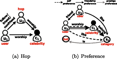

  

  Illustrative examples of hop and preference

  Figure 3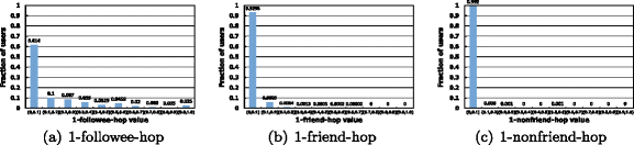

  

  The followship of the same celebrities

  Figure 4a and b show the distributions of user fraction under self-preference and friendship-preference. Surprisingly, these two distributions are so different. The fraction of users that follow big proportion of celebrities who belong to the same categories is large. Conversely, seldom users follow the celebrities who belong to same categories as users’ friend preference. It seems that users pay more attention to self-preference than to friendship-preference. Finally, we also draw the distribution of prestige-preference in Figure 4c. Clearly, the popularity of celebrity categories is not the same, which confirms our expectation. Most users like to follow hot categories such as actors and singers.

Figure 4

The followship of the same categories

2.2.4 The number of followers and the number of followees

As shown in Figure 5, we also illustrate the distribution on users’ number of followers and the number of followees. Obviously, users with a huge number of followees have only a few followers. Conversely, users followed by abundant amount of users follow a small number of users. The result can conclude one important fact that users only track the news of people they are really interested in. Therefore, people who follow a lot of users do not draw much attention from their followees.

Figure 5

The number of followers and the number of followees

Observation summaries

As aforementioned, previous work tend to use the user friendship as the basic concept to predict network links. Based on our observations on hop, preference, and the number of followers/followees, we find that such assumption cannot hold in worship prediction. The observation can be concluded as below. First, the followee-hop has a bigger impact than that of friend-hop and nonfriend-hop on the worship links. Second, the preference analysis shows that users pay more attention to self-preference than to friendship-preference. In addition, the prestige-preference analysis shows that users like celebrities who belong to hot categories. Finally, users who follow a lot of users cannot draw attention from their followees. Therefore, according to these new observations, we can generate appropriate relational properties for worship prediction.

3 Methodology

From the observations mentioned in the previous section, we define several new relational properties such as 1-followee-hop, 1-celebrity-hop, self-preference category, and prestige-preference category. As such, we try to predict which celebrity a user may worship by using these new properties. The flowchart of our framework is shown in Figure 6. At first, a relational property based factor graph (RPG) is proposed to characterize the relations between predicted labels and properties. In addition, we describe a Gaussian estimation based learning algorithm to learn the model parameters to precisely predict worship links between users and celebrities. Finally, an active learning method is also applied to refine our network graph for better accuracy performance.

Figure 6

The overview of our framework

3.1 Relational property based factor graph

We propose a probabilistic graphical model, relational property based factor graph (RPG), to predict the label set $\mathcal {Y}$ for the worship links in the network $\mathcal {G}$. With the relational properties of worship links, our goal is to train this model by using unsupervised learning. As shown in Figure 7, we design the RPG with three kinds of variables (property $\mathcal {R}$, worship $\mathcal {Y}$, and list $\mathcal {T}$) and factor functions (individual factor $\mathcal {P}(y_{i}|\mathcal {R})$, common factor $\mathcal {P}(y_{i}|\mathcal {R}_{(u_{j},c_{k})})$, and list factor $\mathcal {P}(y_{i}|\mathcal {T})$).

• Property: We define a variable set $\mathcal {R}$ which contains the relational properties r_i of worship links. These properties include the statistical properties of user followee, celebrity category, 1-followee-hop, 1-celebrity-hop, self-preference category, and prestige-preference category.

• Worship: The variable set $\mathcal {Y}$ denotes the labels of all worship links to be predicted in this network. These links either are present ($y_{u_{j}\rightarrow c_{k}}= 1$) or are absent ($y_{u_{j}\rightarrow c_{k}}= 0$) in the real world. Worship y_i can be regarded as a label of worship relation $(u_{j} \xrightarrow {{w}} c_{k})$.

• List: The variable set $\mathcal {T}$ represents the worship lists of users. Every variable list t_i = {c_i,1,c_i,2,...,c_i,n} contains celebrities which user u_i may worship.

Figure 7

An illustrative example of RPG

In the probabilistic theory and its applications, factor graphs are used to represent factorization of a probability distribution function [15]. With these three variable sets, we define the following factor functions to compute the desired probability distribution function enabling the worship link prediction.

• (1) Individual factor: The individual factor function draws node properties of worship links such as the number of user followers. Variables property $\mathcal {R}$ and worship $\mathcal {Y}$ are connected by this function, which can be formalized as a conditional probability $\mathcal {P}(y_{i}|\mathcal {R})$ of label y_i by giving properties $\mathcal {R}$. In this work, we model the probability distribution function by Markov random fields [12], which states that a probability distribution with positive density satisfies the Markov properties. The density of the probability distribution can factorize the variables of RPG. Thus, the factor function $\mathcal {P}(y_{i}|\mathcal {R})$ can be defined as a linear exponential function.

  $$ \mathcal{P}(y_{i}|\mathcal{R})=\frac{1}{\mathcal{Z}_{\alpha}}\exp\{\alpha \cdot f(\mathcal{R},y_{i})\}, $$

  (2)

  where the parameters α and $\mathcal {Z}_{\alpha }$ are the corresponding weights, and the normalization factors of the factor functions respectively. Specifically, the function $f(\mathcal {R},y_{i})$ consists of the following subfunctions.

  User Followees (UF)::

  this function U_F(u_j) is the number of user followees. The need of this property comes from the phenomenon that users with huge number of followees have only a few followers. The observation has been discussed in Section 2.2. From this observation, we believe that the number of user’s followees can influence his/her tendency to follow a celebrity. For example, as shown in Figure 1, user u₁ has two followees, and U_F(u₁) = 2.

  Prestige-Preference (PP)::

  P_P(c_k) is defined as the average followers of celebrities who belong to the same category as that of celebrity c_k. The concept of this function is examined by the analysis of ‘prestige-preference’, which implies that users tend to like celebrities belonging to a hot category. As shown in Figure 1, celebrities c₁,c₂ and c₃ in this network are labeled as the same category k₁. Suppose that celebrities c₁,c₂, and c₃ have 100, 200, and 300 followers respectively, the average number of their followers is 200, and P_P(c₁) = 200.

• (2) Common factor: Different from the individual factor, the common factor function refers to the link properties of worship links, which also links variables $\mathcal {R}$ and $\mathcal {Y}$ in RPG. Similarly, this factor function is defined as

  $$ \mathcal{P}(y_{i}|\mathcal{R}_{(u_{j},c_{k})})=\frac{1}{\mathcal{Z}_{\beta}}\exp\{\beta \cdot g(\mathcal{R}_{(u_{j},c_{k})},y_{i})\}, $$

  (3)

  where β is the corresponding weights, $\mathcal {Z}_{\beta }$ is the normalization factors, and function $g(\mathcal {R}_{(u_{j},c_{k})}, y_{i})$ contains three subfunctions as below.

  Followee-Hop(FH)::

  Function F_H(u_j,c_k) refers to the number of 1-followee-hop between a user and a celebrity. The concept is observed from the analysis of ‘1-Followee-Hop’, which shows that a user likes to follow celebrities who are also followees of the user’s followees. For example, as shown in Figure 1, u₂ follows u₃, and c₄ is worshiped by u₂ and u₃. Therefore, F_H(u₂,c₄) = 1.

  Celebrity-Hop(CH)::

  Function C_H(u_j,c_k) represents the number of 1-celebrity-hop between a user and a celebrity. The concept is similar to that of ‘1-Followee-Hop’ function. For example, as illustrated in Figure 1, u₁ worships both c₁ and c₂, and c₁ follows c₂. Therefore, C_H(u₁,c₂) = 1.

  Self-Preference(SP)::

  Function S_P(u_j,c_k) is 1, if celebrity c_k belongs to the preferred categories of user u_j. The definition is from the analysis of ‘Self-Preference’, which indicates that a user likes the same category of celebrities. For example, if user u₁ tends to like the celebrities with category k₁, and u₁ follows c₁ who belongs to k₁. Thus, S_P(u₁,c₁) = 1.

• (3) List factor: This factor function is used to evaluate the correctness of predicted celebrity list, and is defined as

  $$ \mathcal{P}(y_{i}|\mathcal{T})=\frac{1}{\mathcal{Z}_{\gamma}}\exp\{\gamma \cdot h(\mathcal{T},y_{i})\}, $$

  (4)

  where γ and $\mathcal {Z}_{\gamma }$ are the corresponding weights and the normalization factors, respectively.

We use bit vectors $l_{u_{j}}$ and $I_{u_{j}}$ associated with celebrity IDs to record the predicted celebrity list and real celebrity list of user u_j, respectively. The length of $l_{u_{j}}$ is $|\mathcal {C}|$, and the k-th bit of $l_{u_{j}}$ is 1 if and only if the worship link between user u_j and celebrity c_k is predicted as true. List factor function is designed to formalize how close they are for the predicted celebrity list $l_{u_{j}}$ and the real celebrity list $I_{u_{j}}$ of user u_j. As such, function $h(\mathcal {T},y_{i})$ can be defined as follows.

$$ h(\mathcal{T},y_{i})= 1- \frac{\sum \limits_{k = 1}^{|I_{u_{j}}|} (D_{y_{i}}\lbrack k\rbrack)}{|I_{u_{j}}|}, D_{y_{i}}=(l_{u_{j}} \hspace{1ex} XOR \hspace{1ex} I_{u_{j}}), $$

(5)

where XOR is the bitwise ‘XOR’ operation. Generally, $0\leq h(\mathcal {T},y_{i}) \leq 1$. If the accuracy of the predicted list is 100%, $D_{y_{i}}= 0^{T}$ and $h(\mathcal {T},y_{i})= 1$.

However, the exclusive or vector $D_{y_{i}}=(l_{u_{y_{i}}} \hspace {1ex} XOR \hspace {1ex} I_{u_{y_{i}}})$ is actually sparse, and should be designed for running in time proportional to the number of 1 bits. Therefore, a mystical operator ($D_{y_{i}}$ AND ($D_{y_{i}}-1$)) is used to iteratively sets the rightmost 1 bit in $D_{y_{i}}$ to 0.

Factor graphs can be combined with message passing algorithms to efficiently compute the unknown parameters of the function as marginal distributions [15]. Therefore, given all these proposed factor functions which describe the relations among variables, the marginal distribution can be derived as

$$\begin{array}{@{}rcl@{}} \mathcal{P}(\mathcal{R},\mathcal{R}_{(u_{j},c_{k})},\mathcal{T})&=&\prod \limits_{i} \mathcal{P}(y_{i}|\mathcal{R}) \cdot \mathcal{P}(y_{i}|\mathcal{R}_{(u_{j},c_{k})}) \cdot \mathcal{P}(y_{i}|\mathcal{T})\\ &=&\frac{1}{\mathcal{Z}}\prod \limits_{i} \exp \{\theta \cdot (f(\mathcal{R},y_{i}), g(\mathcal{R}_{(u_{j},c_{k})},y_{i}),h(\mathcal{T},y_{i}))\}\\ &=&\frac{1}{\mathcal{Z}}\exp \left\{\theta \cdot \sum \limits_{i} q_{i}\right\}=\frac{1}{\mathcal{Z}}\exp \{\theta \cdot Q\}, \end{array} $$

(6)

where $q_{i} =\{ f(\mathcal {R},y_{i}),g(\mathcal {R}_{(u_{j},c_{k})},y_{i}), h(\mathcal {T},y_{i}) \}, \theta =\{\alpha ,\beta ,\gamma \}$. and $\mathcal {Z} = \mathcal {Z}_{\alpha } \cdot \mathcal {Z}_{\beta } \cdot \mathcal {Z}_{\gamma }$.

In addition, a popular message passing algorithm on factor graphs is the sum-product algorithm [15], which efficiently computes all the marginals of the individual variables of the function. Therefore, the probability of marginal variable y_i is derived as

$$ \mathcal{P}(y_{i}= 1)= \sum \limits_{n} \mathcal{P}(\mathcal{R},\mathcal{R}_{(u_{j},c_{k})},\mathcal{T},y_{n}), y_{n} \in \mathcal{Y}-\{y_{i}\}. $$

(7)

This marginal probability $\mathcal {P}(y_{i}= 1)$ shows that how likely a user u_j worships a celebrity c_k.

3.2 Gaussian estimation based learning

In this section, we introduce the unsupervised method to calculate the weight parameters 𝜃 in the probabilistic function $\mathcal {P}(\mathcal {R},\mathcal {R}_{(u_{i},c_{j})},\mathcal {T})$. To obtain these parameters of RPG, the methodology of Gaussian estimation based learning is utilized. We perform an iterative least-squares fit of unconstrained Gaussian peaks to the relational property data. For the better illustration, we demonstrate a segment of our fitting result as shown in Figure 8. These discovered peaks which fit a portion of data have only a small fitting error of 6.465% with 8 peaks. The observation shows that it is applicable to model the distribution of function set q_i as a summation of several Gaussian distributions:

$$ \mathcal{P}(q_{i})= \sum \limits_{j} a_{j} \mathcal{N}(q_{i}|\mu_{j}, \sigma_{j}), $$

(8)

where μ_j,σ_j, and a_j are the mean, covariance, and coefficient of each Gaussian distribution $\mathcal {N}$, respectively. In addition, j is the number of Gaussian distributions, and the equation ${\sum }_{j} a_{j}= 1$ holds.

Figure 8

The Gaussian peaks of relational properties

As proved in [9], the logarithm of a function achieves its maximum value at the point same as the function itself, and hence the log-likelihood can be used in place of the likelihood in maximum likelihood estimation. For ease of calculation, the distribution function of relational properties discussed in equation (8) is derived as the log-likelihood form:

$$\begin{array}{@{}rcl@{}} ln\ \mathcal{P}(Q)&=& ln \underset{i}{\prod}\left\{\sum \limits_{j} a_{j} \mathcal{N}(q_{i}|\mu_{j},\sigma_{j})\right\}\\ &=&\sum \limits_{i} ln \left\{\sum \limits_{j} a_{j} \mathcal{N}(q_{i}|\mu_{j},\sigma_{j})\right\}. \end{array} $$

(9)

Furthermore, the objective function of this likelihood can be maximized as

$$ \mathcal{O}(\theta)=\underset{\theta}{\arg\max} \prod \limits_{j = 1}^{|Q|} \sum \limits_{y_{i}\in \mathcal{Y}}\mathcal{P}(\mathcal{X}=q_{j},\mathcal{Y}=y_{i}|\theta). $$

(10)

Due to the absence of labels, we use an EM (Expectation-Maximization) algorithm [6] to achieve the maximization of the objective function iteratively.

The EM algorithm is an iterative algorithm that starts from some initial estimate of 𝜃 (e.g., random), and proceeds to iteratively update 𝜃 until the convergence is detected. Specifically, each iteration includes two major steps:

• 1E-step: We fix all model parameters 𝜃 and update latent variables $\mathcal {M}$ by using the gradient descent method:

  $$ \mathcal{Q} (\theta,\theta_{old})=\sum \limits_{\mathcal{M}} \mathcal{P}(\mathcal{M}|\mathcal{X},\theta^{old}) \ln \mathcal{P}(\mathcal{X},\mathcal{M}|\theta), $$

  (11)

  where $\mathcal {M}$ is the latent variables in this EM model. Latent variables are variables that are not directly observed but are rather inferred from other variables that are observed.

• 2.M-step: All latent variables $\mathcal {M}$ are fixed and each model parameter 𝜃 is updated in this step.

  $$ \theta^{new}=\underset{\theta}{\arg\max} \mathcal{Q} (\theta,\theta^{old}). $$

  (12)

In the EM model, we first compute the distribution probability of relational property data. Given all data points q_i,1 ≤ i ≤ n and K Gaussian components, the probability γ(i,k) of a data point q_i assigned to component k is

$$ \gamma(i,k)=\frac{a_{k} \mathcal{N}(q_{i}|\mu_{k},\sigma_{k})}{\sum \limits_{j = 1}^{K} a_{j} \mathcal{N}(q_{i}|\mu_{j},\sigma_{j})}. $$

(13)

Based on the foregoing, we use the updated γ(i,k) to compute new μ_k and σ_k as below.

$$ \mu_{k}=\frac{1}{N_{k}}{\sum}_{i = 1}^{n}\gamma(i,k)\cdot q_{i}, $$

(14)

and

$$ \sigma_{k}=\frac{1}{N_{k}}{\sum}_{i = 1}^{n}\gamma(i,k)(q_{i}-\mu_{k})(q_{i}-\mu_{k})^{T}, $$

(15)

where $N_{k}={\sum }_{i = 1}^{n}\gamma (i,k)$.

Overall, these equations need to be computed in this order: first we enumerate the K new γ, the K new μ_k, and finally the K new σ_k. The E-M steps are repeated in this manner until reaching the convergence. After the parameters are acquired, we will have $\mathcal {P}(y_{i}= 1)$, for each $y_{i}\in \mathcal {Y}$.

3.3 Active learning

The unsupervised learning method, RPG with Gaussian estimation based learning, has quite high accuracy, which will be shown in the experimental results. However, it is worth reaching a better accuracy performance by querying only a small set of labels. Considering the interactive user queries of social systems [28, 30], we intend to apply the concept of active learning in our framework. Active learning (AL) algorithms enable actively query the user/expert for only a small set of labels. Therefore, the key factor that contributes to the success of active learning lies in querying the most effective link to be labeled, which can significantly enhance the performance of our system. The active learning process is designed to be an iterative process including two phrases: (1) Link Selection, and (2) Graph Refinement.

• (1) Link Selection: The active learning is designed to select one link for labeling in each iteration. Due to the limitation of human resources, we can select only n links in total, where n is supposed to be a small value. To be more effective, we propose four selection strategies.

  Random: :

  We randomly pick one link for labeling, which means that any link has the same probability to be chosen in each iteration.

  Positive: :

  Intuitively, a link $e_{u_{i}\rightarrow c_{j}}$ with the highest probability of being positive has a great confidence. However, if a negative feedback is obtained, we can certainly know that celebrity c_k has the unfavorable side-effect on the link prediction with user u_j. In each iteration, we select the unlabeled link with the highest probability of being positive as the labeling candidate l_c, which can be formulated as

  $$ l_{c}=\underset{y_{i}}{\arg\max} \mathcal{P} (y_{i}= 1). $$

  (16)

  Negative: :

  In this strategy, we select the unlabeled link with the highest probability of $\mathcal {P} (y_{i}= 0)$ as the labeling candidate l_c, which can be formulated as

  $$ l_{c}=\underset{y_{i}}{\arg\max} \mathcal{P} (y_{i}= 0). $$

  (17)

  In this case, if a positive feedback is obtained, celebrity c_k may actually have good effect on the link prediction of user u_j. The reason comes from the fact that connection between celebrity c_k and user u_j can help user u_j to reach more potential worship links through celebrity c_k.

  Uncertain: :

  The probability $\mathcal {P} (y_{i})$ reflects the potential of a worship link to be positive or negative. Those links with the lowest proximity scores are supposed to be the most uncertain ones. It’s reasonable that labeling the uncertain links would enhance the performance of our framework.

  $$ l_{c}=\underset{y_{i}}{\arg\min} \mathcal{P} (y_{i}). $$

  (18)

• (2) Network Refinement: With the user feedback, we try to refine the original network graph, which can help to achieve the more accurate RPG in each iteration. More specifically, we design an algorithm to delete nodes or create links according to these obtained labels. The detailed process is described as follows.

  False Positive (FP) cases: :

  In this case, a negative user feedback is returned when a positive label of link $e_{u_{i}\rightarrow c_{j}}$ is predicted. In other words, our system identifies that user u_j has a close relation with celebrity c_k, which is an incorrect result. In addition, this link $e_{u_{i}\rightarrow c_{j}}$ may further lead the user node u_j to reach other nodes through this link [21]. To avoid such a case, we remove the celebrity node c_k from the original network graph. Such removal will prohibit user u_j suffering from reaching the neighbors of c_k.

  False Negative (FN) cases: :

  We create a link to connect the query user u_j and celebrity c_k, if link $e_{u_{j}\rightarrow c_{k}}$ gets the positive labeling feedback. Myers et al. [24] identified that the inbound one-hop neighborhood of a user can increase the information dissemination potential of this user.

  True Positive (TP) cases: :

  Similarly, when the system correctly predicts the positive label of link $e_{u_{j}\rightarrow c_{k}}$, the link should be added to the network. As such, this new link will help user u_j to approach more worship links with other celebrities by celebrity c_k [21].

  As regards to True Negative (TN) cases, the system will not make any refinement on the given network. After the link creation/deletion in each iteration, the revised network graph needs to be retrained by Gaussian estimation based learning methods to enhance the accuracy performance of our model.

4 Experimental results

This section presents experimental studies of this research. All the data are crawled using the PHP language. In addition, all the network analysis and prediction algorithms are programed in Python on a PC running Ubuntu 14.04 with 3.40 GHz Core i7 CPU and 16GB RAM.

4.1 Experimental setup

4.1.1 Datasets

Three kinds of real datasets are used to verify our system in experiments, including Twitter, DBLP, and Instagram data. The detailed information of these datasets is shown in Table 1.

Table 1 Statistics of Instagram, Twitter, and DBLP datasets

Instagram dataset

As we mentioned in Section 2.2.1, our collected Instagram data is crawled by Instagram API. To identify whether a user is a celebrity, we try to query his/her full name in DBpedia,³ representing his/her information is indexed in the Wikipedia knowledge base. Almost 4.4% Instagram users are identified as celebrities. Using the same way, we can also query the career category of a celebrity. Finally, almost 100,000 nodes, 3,000,000 links, and 15 categories are obtained to produce the Instagram celebrity-dived network.

DBLP dataset

This dataset contains citation data which is extracted from DBLP [31]. We use almost 100,000 papers and 1,000,000 citations to generate the desired DBLP network. Each paper is associated with abstract, authors, year, venue, and title. The top 4.4% papers with a large amount of citations are identified as celebrities in this network. To discover the categories of celebrities, we retrieve the keywords from paper titles by frequent pattern mining [1]. Finally, 12 kinds of categories are defined.

Twitter dataset

In social network websites, we use Twitter data which is collected from [11]. Twitter is an online news and social networking service where users post and read messages. In this study, almost 110,000 users and 8,200,000 ‘follow’ links are used to generate the twitter network. Similar to the case of DBLP, we identify the top 4.4% users with many followers as celebrities and retrieve 18 terms as celebrity categories by text mining.

4.1.2 Evaluation metrics

In this paper, we use four evaluation metrics for different purposes.

Precision

Precision in this paper is the fraction of the predicted positive links L_p that are relevant to the real positive links L_r. It cares about the probability that real positive links can be discovered by our system. The precision is defined as $\frac {|L_{p}\cap L_{r}|}{|L_{p}|}$.

AUC

To consider both measures of recall and precision, AUC in this paper represents the area under the Precision and Recall (PR) curve [5]. AUC can be any value between 0 and 1, where a bigger value suggests the better overall performance of a prediction system.

RMSE

The root-mean-square error (RMSE) [14] is a frequently used measure of the differences between values estimated by a model and the values actually observed. In this paper, the RMSE can be defined as $\sqrt {\frac {{\sum }_{i = 1}^{n} (\hat {y_{i}}-y_{i})^{2}}{n} }$, where $\hat {y_{i}}$ is the predicted label, y_i is the true label, and n is the number of total worship links.

NDCG

The normalized discounted cumulative gain (NDCG) is a measure of ranking quality [14], which is often used to measure effectiveness of search results in information retrieval. The concept of DCG comes from that highly relevant documents are more useful when appearing earlier in a search engine result list. In this paper, the DCG can be defined as ${\sum }_{i = 1}^{p} \frac {rel_{i}}{log_{2}i}$, where rel_i is the graded relevance of the predicted label y_i at position i of the predicted results ordered by the predicted probability, and p is the number of predicted links.

4.1.3 Methods for comparisons

Three relational property based methods and four state-of-the-art methods of unsupervised learning which can be used to predict our desired links are described as below.

Hop (H)

To understand the effect of hop based properties, we use only ‘1-Followee-Hop’ and ‘1-Celebrity-Hop’ functions in this method by applying the proposed framework.

Preference (P)

Similarly, we try to use the relational properties, including ‘Prestige-Preference’ and ‘Self-Preference’, on RPG to see the effect of preference.

Follower-Followee (FF)

In this case, we only focus on the function drawing relations between Follower and Followee, which refers to the ‘User Followees’ function.

User Friendship (UF)

Traditional link prediction methods like to use the factor of user friendship to predict the label [8, 17, 36, 37]. Therefore, in this work, we also try to use relational properties with respect to the previous work. As such, the properties of ‘one-friend-hop’, ‘self-preference’, and ‘friendship-preference’ are applied on the RPG to predict the worship links.

Preferential Attachment (PA)

One well-known concept in social networks is that users with many neighbors tend to create more connections in the future. This is due to the fact that in some social networks, like in finance, the rich get richer. Therefore, we try to estimate how “rich” two vertices are by calculating the multiplication between the number of followers each vertex has. The prediction score of preferential attachment for any worship link $e_{u_{i}\rightarrow c_{j}}$ is defined as |N(u_i)|×|N(c_j)|, where N(u_i) is the neighbor set of user u_i.

Jaccard Coefficient (JC)

Jaccard coefficient is a measurement of asymmetric information on two nodes in a network graph. The prediction score of Jaccard coefficient for any worship link $e_{u_{i}\rightarrow c_{j}}$ can be computed using set relations $\frac {|N(u_{i})\cap N(c_{j})|}{|N(u_{i})\cup N(c_{j})|}$.

Betweenness Centrality (BC)

Betweenness centrality is a measure of centrality in a graph based on shortest paths. For every pair of vertices in a graph, there exists a shortest path between the vertices. The betweenness centrality for each link is the number of these shortest paths that pass through the link. As a result, we can define this prediction value of any worship link $e_{u_{i}\rightarrow c_{j}}$ as ${\sum }_{s\neq t\neq u_{i}\neq c_{j}}\frac {\sigma _{s,t} (e_{u_{i}\rightarrow c_{j}})}{\sigma _{s,t}}$, where σ_s,t is the number of shortest paths between nodes s and t that pass through the link $e_{u_{i}\rightarrow c_{j}}$.

4.2 Evaluation of RPG

In this section, we discuss the accuracy performance of the proposed RPG, comparing with other methods in different networks. More specifically, we sample 75% network data as a training set, while holding out 25% of the data for testing our model. The accuracy performance reported by 4-fold cross-validation is then the average of the accuracy values computed in each training and testing phase.

4.2.1 Comparison with previous work

The accuracy results of all methods applied on Instagram are shown in Table 2. We first compare the performance of our method with previous work such as preferential attachment, Jaccard coefficient, betweenness centrality, and user friendship by precision, AUC, RMSE, and NDCG. The RPG method is to exploit Gaussian based learning on RPG without active learning.

Table 2 Accuracy performances of all methods on Instagram data (in percentage)

From these results, we have the following observations. First, the accuracy of the RPG algorithm outperforms all the other methods. The accuracy differences of precision, AUC, and NDCG between our method and previous work are [15% − 28%], [8% − 14%], and [(− 0.22)% − 4.98%], respectively, which are huge gaps. As regards to the ranking quality of the predicted result, we rank predicted labels based on their predicted probabilities, and compare the rankings with the ground-truths to obtain AUC and NDCG scores. Therefore, the good accuracies on AUC and NDCG prove that highly relevant links appear earlier in our predicted list, which shows the ranking effectiveness of our method. Finally, as the concern of prediction errors, RPG has the smallest RMSE among these methods.

On the other hand, the accuracy of all methods, excluding RPG, are close to each other. The overview of their performance is that the accuracy of JC would be higher than that of PA, BC, and UF in order. All of their precisions are not over 70%, which means that more than 30% of their generated worship links are unconvincing. The reasons can be drawn that these previous methods do not consider the factor of hops and preferences.

4.2.2 Comparison with different relational properties

We also discuss the accuracy performances of different relational properties such as hop, preference, and follower-followee. Obviously, RPG has the best accuracy performance comparing to using different relational properties, which is shown in Table 2. Among these properties used in RPG, hop and follower-followee refer to the most and the least important factor to affect the accuracy of RPG, respectively. Surprisingly, using the properties of hop or preference enables a more effective model than that of previous work. However, only the factor graph with all these properties can reach the highest accuracy.

4.2.3 Effect of different networks

Furthermore, as shown in Tables 3 and 4, we exam the accuracy performances of all methods on different networks, Instagram, Twitter, and DBLP. As we can expect, these methods have varied accuracy performances on different networks, since each network has its own social properties. Surprisingly, RPG is still the top 1 of all methods, which can retrieve precise worship links. Overall, the best performance of RPG occurs on DBLP, followed by Instagram and Twitter. The accuracy performances of other methods on different networks are variant. For example, PA and BC can have a very low accuracy on DBLP, which is different from the status on Twitter and Instagram. On the other hand, UF has the similar precisions which are averaged as 53.85% on different networks. Moreover, hop and preference can discover very high quality links on DBLP.

Table 3 Accuracy performances of all methods on DBLP data (in percentage)

Table 4 Accuracy performances of all methods on Twitter data (in percentage)

Overall, we can conclude that the RPG algorithm is able to retrieve not only accurate worship links but also the ones with high ranking qualities in different networks.

4.3 Evaluation of active learning

In this section, we further demonstrate the accuracy performance of all methods with active learning. Since these methods applied for comparison are unsupervised learning, we can implement an active learning process for each of them.

4.3.1 Comparison with previous work

The precision results and the improvements by active learning of all previous work applied on Instagram are shown in Table 5. It is clear that the accuracy performances of most methods can be enhanced by active learning, since most improvements are positive. However, the precision of RPG with active learning still outperforms the previous work with active learning. The precision differences of four selection strategies between our method and previous work are ranging from 2.8% to 40.76%, which are huge gaps.

As aforementioned, active learning is an iterative process, and the number of iteration (the number of queried labels for each user) can definitely influence the precision of predicted results. Therefore, we vary the number of iteration n, and illustrate the trends of precision results for previous work in Figure 9. Note that the precision curve of RPG on different number of iterations is shown in Figure 11a. Obviously, more iterations can lead to a higher precision of a method. It is reasonable that the more true labels we can obtain, the more accurate model we can have. Moreover, for a small number of iterations, the precision is increasing with the significant difference. However, when the number of iterations is getting bigger, the precision is increasing in an ignorable difference.

4.3.2 Comparison with different relational properties

We further discuss the precision results of different properties with active learning. As shown in Table 5, RPG has higher accuracy, comparing to hop, preference, and FF. Considering these properties used in RPG, the accuracies of preference and FF can be highly improved by active learning. However, hop is the most effective method among these properties without active learning.

Table 5 Accuracy performances and improvements of all methods with active learning (precision in percentage)

Therefore, we illustrate the precision trend of active learning in Figure 10. From these results, we have the following observations. First, the increasing curve (positive selection) of hop is growing much slower than the ones of preference and FF. The reason may come from the fact that preference and FF have lower accuracy before active learning, and they can be easily enhanced by querying wrongly predicted labels for network refinement.

4.3.3 Effect of different networks

To exam the stability of our framework on different networks, we apply RPG with active learning on Instagram, Twitter, and DBLP. As shown in Table 6, the active learning obviously enhances the accuracy performance of our model on different datasets. For the DBLP data, our method can even approach the best precision of 100%. As regards to the Instagram data, the active learning phase improves the accuracy at most 13% precision to reach a very high precision as almost 96%. In addition, the accuracy of Twitter data cannot be improved as much as that of other networks,

Table 6 Accuracy performances of our framework in different networks (precision in percentage)

We further illustrate the precision trend of active learning in Figure 11 for these networks. From these results, we have the following observations. First, more iterations can lead to a higher precision of a method, and the curve of DBLP reaches 100% on the third iteration. Moreover, for a small number of iterations, the precision is increasing with the significant difference. However, when the number of iterations is getting bigger, the precision is increasing in an ignorable difference. Finally, the increasing curves of Instagram and Twitter are so similar, which shows the stability of our method. Due to the space limitation, the active learning performances of other methods on Twitter and DBLP are not demonstrated. However, the performance of active learning applied on Instagram is similar to that on Twitter and DBLP data.

4.3.4 Effect of different selection strategies

Finally, we focus on the issue of selection strategies. As shown in Figures 9, 10, and 11, different selection strategies have the variant performance for different methods. Overall, the uncertain selection is suitable for RPG and PA. The reason can be drawn that the network graph of RPG and PA can be largely refined from the most uncertain candidates with the lowest proximity scores. On the other hand, JC, BC, and UF need the random strategy to have their best performance, so the appropriate candidates to enhance the accuracy are not based on the predicted probability. The positive one can highly improve the accuracy of Hop, Preference, and FF. Finally, no matter the refinement phase refers to the false positive or true positive case, the network can be modified to be a better RPG model.

Figure 9

Accuracy performances of previous work with active learning (on Instagram)

Figure 10

Accuracy performances of relational properties with active learning (on Instagram)

Figure 11

Accuracy performances of RPG with active learning on different networks

Surprisingly, the negative selection does not work well in every method. For false negative cases in negative selection, we create links to connect the query user u_j and celebrity c_k. However, those added links cannot help users to approach more precise worship links, which is not as we expect. Moreover, not every selection strategy enables to improve the accuracy of methods without active learning.

4.4 Execution time analysis

In this section, we discuss the execution time of all these comparing methods.

4.4.1 The execution time of unsupervised methods

First, we demonstrate the execution time of different methods without active learning on Instagram data, which is shown in Figure 12a. Obviously, the efficiency ranking of these methods is FF, Preference, RPG, Hop, UF, JC, PA, and BC, in sequence. This figure is plotted in log scale. The execution time of RPG, Hop, Preference, and FF is 2-3 orders of magnitude faster than that of previous work. More specifically, the time difference of previous work and RPG is from minutes to hours. On the other hand, the execution time of FF and Preference is a little shorter than that of RPG, since RPG considers all properties. However, FF and Preference obtain lower accuracy, which makes the RPG the best solution we have.

Figure 12

The execution time analysis of unsupervised methods and active learning

4.4.2 The execution time of active learning

We also demonstrate experiments on the execution time of two phases in our framework including RPG and AL (10 iterations). As illustrated in Figure 12b, the AL process, including link selection and graph refinement, takes the most time in our framework, since the AL process iteratively retrains the model. And the execution time differences between AL phase and these unsupervised methods are 2 − 3 orders of magnitude. Furthermore, the efficiency ranking of these methods with AL is the same as that of the methods without AL. It is reasonable that these methods are repeatedly executed in each iteration of their AL processes.

4.4.3 The execution time of selection and refinement

We discuss the execution time of selection and refinement phases in active learning, which is shown in Figure 13a. It is clear that the execution time of selection and refinement is in direct proportion. In addition, the refinement needs more time than that of selection phase, and the time difference between these two phases is 1 − 4 orders of magnitude. The reason comes from the fact that the refinement contains the retraining part of each model.

Figure 13

The execution time analysis of active learning

4.4.4 Effect of different selection strategies

Different selection strategies are variant not only on accuracy performance but also on efficiency performance for unsupervised methods. From the results illustrated in Figure 14, we have the following observations. First, the uncertain selection on RPG needs more time than other strategies. As aforementioned, RPG can reach the best accuracy performance with the uncertain selection. Therefore, the network graph generated by RPG should be refined the most by choosing uncertain candidates, which lead to the longer processing time of RPG with uncertain selection. In addition, the positive selection takes higher execution time than other strategies in different methods. Finally, though the execution time of different selection strategies is variant, they would not have large difference when applying in the same unsupervised method.

Figure 14

The execution time analysis of selection strategies in active learning

4.4.5 Effect of different networks

The execution time of our framework applied on Twitter, Instagram, and DBLP, is illustrated in Figure 13b. Obviously, the efficiency ranking of our method implemented on different networks is Instagram, DBLP, and Twitter. In general, the execution time is proportional to the scale of a network. Since the Twitter network is larger than that of Instagram and DBLP, the execution time of Twitter is much bigger than the others. In addition, the number of links in Twitter is much bigger than that of other networks, which also causes the long time process of our method on Twitter.

In conclusion, these experimental results indicate that our method is effective and efficient on different networks, which shows the stability of this framework.

5 Related work

In this section, we review previous studies related to link prediction and learning on factor graphs.

Link prediction

Networks have become more and more important in our daily life with the advent of Internet on smart phones, tablets, and computers. Any network can be represented as a graph consisting of nodes (users) and links between the nodes. It is essential to know how new links are added to the network as time advances, which can often refer to the problem of ‘link prediction’ [20, 35]. The real applications of link prediction include recommendation systems, potential customers discovery, domain experts identification, and so on.

The link prediction problem in network industry was early addressed in [10, 20, 25, 29]. Liben-Nowell et al. firstly developed similarity based approaches for analyzing the proximity of links occurring in the future of a network [20]. It presents measures such as node neighborhoods, the ensemble of paths for estimating the similarity of nodes in a social network. Since then, abundant researches based on graph topology have been dedicated to link prediction. PA (Preferential Attachment) [20], JC (Jaccard Coefficient) [20], and CN (Common Neighbors) [25] infer the probability of links by product of the degree of two nodes, the intersection and union of neighbors, and the number of common neighbors of two nodes, respectively. In addition, Haifeng et al. [10] use BC (betweenness centrality) which measures the centrality of shortest paths to solve the hidden link prediction. Similarly, a link between two nodes is predicted based on the probability of information propagation between the two nodes [29].

Recently, researchers develop many unsupervised and supervised learning algorithms for link prediction on varied networks. Pujari et al. [27] presented a supervised rank aggregation approach for link prediction in complex networks. Miller et al. [22] proposed an onparametric Bayesian technique to predict links in relational data. Moreover, with considering the dual graph, link prediction in co-author network can be substantially enhanced [3]. Tasnádi et al. [33] used supervised machine learning techniques and independent information such as ratings and languages used by the users to test the connection of users. Finally, many studies focus on learning with probabilistic models in the literature [8, 17, 36, 37]. Such approaches apply essentially selected features such as friendship of nodes and apply an appropriate probabilistic model with chosen features on social networks for link prediction.

In addition, Ding et al. [7] focus on the celebrity recommendation for users in Tencent and Twitter networks. The authors proposed a unified hierarchical Bayesian model and considered both social ties and descriptions of celebrities to improve the prediction ability and recommendation interpretability. This research leverages the semantic analysis power [4] to solve hard explainability problem existing in the context of matrix factorization. It is necessary to collect abundant personal descriptions of each celebrity from Wikipedia, LinkedIn and their personal websites. In our work, detailed description data of users are not required.

Specifically, the previous work [7] attempts to extract the appropriate user information as features for supervised learning on link prediction. However, user privacy has been recognized as an important issue nowadays, and the assumption that users can provide their detailed information is no longer valid. In addition, we fully explore the new relational properties which have not been utilized in [7]. As will be demonstrated in experimental studies, it is highly useful for link prediction in celebrity-dived networks. Clearly, our work is related but orthogonal to these work in [7].

Factor graphs learning

In probability theory, a factor graph is a bipartite graph which is used to represent factorization of a probability distribution. A well-known method, sum-product algorithm, enables efficient computations of learning on factor graphs [16]. Recently, factor graphs have been used to resolve various problems [8, 13, 32, 34]. Considering the issue of time constraints, Wang et al. [34] developed an unsupervised factor graph to predict the relationship between advisor and advisee. In addition, John et al. [13] proposed a factor graph model, TriFG, with social ties of users to predict the reciprocal relationship between users. In [32], the authors use the factor graph to infer social ties across heterogeneous networks. Finally, to solve the link prediction in coupled networks, a coupled factor graph model incorporating the meta-paths extracted from the coupled part of the two networks is designed for transferring heterogeneous knowledge [8]. However, these proposed methods do not consider the statistical properties of nodes.

6 Conclusions

We in this paper explore a new link prediction paradigm, called ‘Worship link prediction’, to discover worship links on celebrity-dived networks. We also observe interesting user worshiping behavior based on hops and preferences in social services, which motivates exploring new relational properties for link prediction algorithms. With the concern of business security and personal privacy, we use statistical relational properties, instead of the detailed information of users, to predict the ‘worship’ labels.

To address these issues, a novel factor graph RPG with new discovered statistical properties is proposed. In addition, we also design a Gaussian estimation based learning algorithm to efficiently and effectively discover the ‘worship’ links. To enhance the accuracy performance, an active learning process is devised to refine the network graph by only querying a few labels.

Finally, the proposed framework is implemented with empirical studies on real data, Instagram, Twitter, and DBLP in order to gain insights into the accuracy of predicted links. The results show that our framework achieves good stability. Moreover, different types of methods are discussed in this paper, which shows the incapability of previous work. As regards to the efficiency performance, our framework can save a huge amount of time in the learning process, compared with the traditional link prediction methods.

References

Agrawal, R., Srikant, R.: Fast algorithms for mining association rules in large databases. In: VLDB’94, Proceedings of 20th international conference on very large data bases, September 12-15, 1994, Santiago de Chile (1994)
Barbieri, N., Bonchi, F., Manco, G.: Who to follow and why: link prediction with explanations. In: KDD (2014)
Benchettara, N., Kanawati, R., Rouveirol, C.: A supervised machine learning link prediction approach for academic collaboration recommendation. In: RecSys (2010)
Blei, D. M., Ng, A. Y., Jordan, M. I.: Latent dirichlet allocation. Journal of machine Learning research (2003)
Davis, J., Goadrich, M.: The relationship between precision-recall and roc curves. In: ICML (2006)
Dempster, A.P., Laird, N.M., Rubin, D.B. : Maximum likelihood from incomplete data via the em algorithm. Journal of the royal statistical society. Series B (methodological) (1977)
Ding, X., Jin, X., Li, Y., Li, L.: Celebrity recommendation with collaborative social topic regression. In: IJCAI (2013)
Dong, Y., Zhang, J., Tang, J., Chawla, N.V., Wang, B.: Coupledlp: Link prediction in coupled networks. In: KDD (2015)
Edwards, A.W.F.: Likelihood CUP archive (1984)
Freeman, L.C.: A set of measures of centrality based on betweenness. Sociometry (1977)
Galuba, W., Aberer, K., Chakraborty, D., Despotovic, Z., Kellerer, W.: Outtweeting the twitterers - predicting information cascades in microblogs. In: Workshop on WOSN (2010)
Hammersley, J. M.: P Clifford Markov fields on finite graphs and lattices (1971)
Hopcroft, J., Lou, T., Tang, J.: Who will follow you back?: reciprocal relationship prediction. In: CIKM (2011)
Hyndman, R.J., Koehler, A.B.: Another look at measures of forecast accuracy. International journal of forecasting (2006)
Kschischang, F.R., Frey, B.J., Loeliger, H.: Factor graphs and the sum-product algorithm. IEEE Trans. Information Theory, (2) (2001)
Kschischang, F.R., Frey, B.J., Loeliger, H.-A.: Factor graphs and the sum-product algorithm. IEEE Transactions on information theory (2001)
Kuo, T. , Yan, R. , Huang, Y., Kung, P., Lin, S.: Unsupervised link prediction using aggregative statistics on heterogeneous social networks. In: KDD (2013)
Lei, S., Maniu, S., Mo, L., Cheng, R., Senellart, P.: Online influence maximization. In: KDD (2015)
Li, J., Zhang, L., Meng, F., Li, F.: Recommendation algorithm based on link prediction and domain knowledge in retail transactions. Procedia Computer Science (2014)
Liben-Nowell, D., Kleinberg, J.: The link-prediction problem for social networks. Journal of the Association for Information Science and Technology (2007)
McPherson, M., Smith-Lovin, L., Cook, J.M.: Birds of a feather: Homophily in social networks. Annual review of sociology (2001)
Miller, K. , Jordan, M.I., Griffiths, T.L.: Nonparametric latent feature models for link prediction. In: Advances in neural information processing systems (2009)
Miyauchi A., Kawase, Y.: What is a network community?: A novel quality function and detection algorithms. In: CIKM (2015)
Myers, S.A., Sharma, A. , Gupta, P., Lin, J.: Information network or social network?: the structure of the twitter follow graph. In: Proc. of WWW (2014)
Newman, M.E.: Clustering and preferential attachment in growing networks. Physical Review E (2001)
Peng, R., Sun, D., Tsai, W.-T.: Success factors in mobile social networking application development: case study of instagram. In: Proc. of SAC (2014)
Pujari M., Kanawati, R.: Supervised rank aggregation approach for link prediction in complex networks. In: WWW (2012)
Rubens, N., Elahi, M., Sugiyama, M., Kaplan, D. : Active learning in recommender systems. In: Recommender systems handbook (2015)
Saito, K., Nakano, R., Kimura, M.: Prediction of link attachments by estimating probabilities of information propagation. In: KES (2007)
Settles, B.: Active learning literature survey. University of Wisconsin, Madison (2010)
Tang, J., Zhang, J., Yao, L., Li, J., Zhang, L., Su, Z.: Arnetminer: extraction and mining of academic social networks. In: KDD (2008)
Tang, J., Lou, T., Kleinberg, J.: Inferring social ties across heterogenous networks. In: WSDM (2012)
Tasnádi, E., Berend, G.: Supervised prediction of social network links using implicit sources of information. In: WWW (2015)
Wang, C., Han, J., Jia, Y., Tang, J., Zhang, D., Yu, Y., Guo, J.: Mining advisor-advisee relationships from research publication networks. In: KDD (2010)
Wang, P., Xu, B., Wu, Y., Zhou, X.: Link prediction in social networks: the state-of-the-art. Science China Information Sciences (2015)
Zhao, T., Zhao, H.V., King, I.: Exploiting game theoretic analysis for link recommendation in social networks. In: CIKM (2015)
Zheleva, E., Getoor, L., Golbeck, J., Kuter, U.: Using friendship ties and family circles for link prediction. In: Advances in social network mining and analysis. Springer, Berlin (2010)
Zimmerman, J., Parameswaran, L., Kurapati, K.: Celebrity recommender. Carnegie Mellon University Research Showcase (2002)
Acknowledgements
This study was supported in part by the Ministry of Science and Technology (MOST) of Taiwan, R.O.C., under Contracts 104-2628-E-001-005-MY3, 105-2628-E-001-002-MY2, 106-3114-E-002-008, and 105-2221-E-006-140-MY2. All opinions, findings, conclusions, and recommendations in this paper are those of the authors and do not necessarily reflect the views of the funding agencies.
Author information
Authors and Affiliations
Corresponding author
Rights and permissions
About this article
Cite this article
Teng, SY., Ting, LPY., Yeh, MY. et al. Worship prediction: identify followers in celebrity-dived networks. World Wide Web 22, 347–373 (2019). https://doi.org/10.1007/s11280-018-0569-y
Received:
Revised:
Accepted:
Published:
Issue Date:
DOI: https://doi.org/10.1007/s11280-018-0569-y