Abstract
It is well-known that the Tucker decomposition of a multi-dimensional tensor is not unique, because its factors are subject to rotation ambiguities similar to matrix factorization models. Inspired by the recent success in the identifiability of nonnegative matrix factorization, the goal of this work is to achieve similar results for nonnegative Tucker decomposition (NTD). We propose to add a matrix volume regularization as the identifiability criterion, and show that NTD is indeed identifiable if all of the Tucker factors satisfy the sufficiently scattered condition. We then derive an algorithm to solve the modified formulation of NTD that minimizes the generalized Kullback-Leibler divergence of the approximation plus the proposed matrix volume regularization. Numerical experiments show the effectiveness of the proposed method.
1. INTRODUCTION
Tensors are multi-dimensional extensions of matrices [1, 2]. The Tucker decomposition [3] of a multiway tensor is perhaps the most natural generalization of the celebrated matrix principal component analysis (PCA) due to its close relationship with the higher-order singular value decomposition (HOSVD) [4, 5]. However, it also inherits the biggest shortcomings of PCA, namely the latent factors are not identifiable due to the inherent rotation ambiguity (without additional constraints on the latent factors). For this reason, the Tucker decomposition is most commonly used as a compression technique rather than an unsupervised factor analysis approach or blind source separation method, unlike most other tensor decomposition models such as the canonical polyadic decomposition [6–10].
Inspired by the success of nonnegative matrix factorization (NMF) [11], there have been nonnegative variants of Tucker decomposition as well [12–15]. Although general matrix factorization is not unique, NMF has been observed to be able to (sometimes, not always) correctly identify the latent factors by simply adding nonnegativity constraints. The most general result to date is that NMF is unique when the latent factors satisfy the ‘sufficiently scattered’ condition [16]. Furthermore, one could enforce the factors to be sufficiently scattered by optimizing a matrix volume criterion [17]. An overview on identifiability and applications of NMF can be found in [18].
In this paper, we make the first ever attempt to extend such identifiability results to nonnegative tensor decomposition (NTD). We will show that NTD is identifiable, up to scaling and permutation ambiguity, if all the factor matrices are sufficiently scattered. Identifiability of NTD is accomplished by optimizing a novel volume criterion imposed on the core tensor. When noise is present, this naturally leads to a volume-regularized NTF model that jointly fits the data and also uniquely identifies the latent factors. Experiments on synthetic and real data validates the effectiveness of our model.
1.1. Tensors and notations
We denote the input -way tensor, of size , as . In general, we denote tensors by boldface Euler script capital letters, e.g., and , while matrices and vectors are denoted by boldface italic capital letters (e.g., and ) and boldface italic lowercase letters (e.g., and ), respectively. The Euclidean norm of a tensor is denoted as , which is defined as
Unfolding.
A tensor can be unfolded, or matricized, along any of its mode into a matrix. The tensor unfolding along the th mode is denoted . More simply, the th mode of forms the rows of and the remaining modes form the columns.
Tensor-matrix product.
The -mode tensor-matrix product multiplies a tensor with a matrix along the th mode. Suppose is a matrix, the -mode tensor-matrix product, denoted as , outputs a tensor of size . Elementwise,
Using mode- unfolding, it can be equivalently written as
Note that the resulting tensor is in general dense regardless of the sparsity pattern of .
A common task is to multiply a tensor by a set of matrices. This operation is called the tensor-times-matrix chain (TTMc). When multiplication is performed with all modes, it is denoted as , where is the set of matrices . Sometimes the multiplication is performed with all modes except one. This is denoted as , where is the mode not being multiplied:
Kronecker product.
The Kroneckder product (KP) of and , denoted as , is an matrix defined as
Mathematically, the -mode TTMc can be equivalently written as the product of mode- unfolding times a chain of Kronecker products:
| (1) |
More notations are shown in Table 1.
Table 1:
List of notations
| Symbol | Definition |
|---|---|
| N | number of modes |
| 𝒳 | N-way data tensor of size I1 × I2 × … × IN |
| 𝒳(i1, …, iN) | (i1, …, iN)-th entry of 𝒳 |
| X (n) | mode-n matrix unfolding of 𝒳 |
| I n | dimension of the nth mode of 𝒳 |
| K n | multilinear rank of the nth mode |
| 𝒢 | core tensor of the Tucker model |
| U (n) | mode-n factor of the Tucker model |
| {U} | set of all factors {U (1), …U (N)} |
| ×n | n-mode tensor-matrix product |
| ×−n | chain of mode products except the nth one |
1.2. Nonnegative Tucker decomposition (NTD)
The goal of Tucker decomposition is to approximate a data tensor with the product of a core tensor and a set of factor matrices , i.e., . An illustration of Tucker decomposition for 3-way tensors is shown in Figure 1. To find the Tucker decomposition of a given tensor with a target reduced dimension , one formulates the following problem:
| (2) |
Fig. 1:
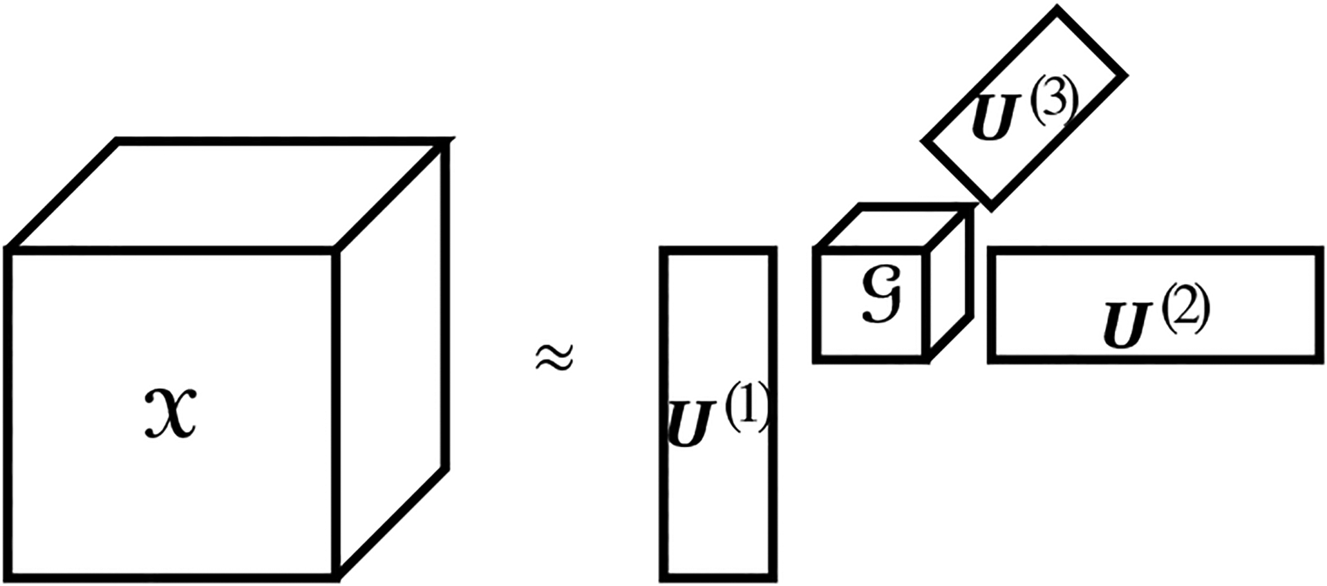
Tucker decomposition of a 3-way tensor
Similar to matrix factorization models, the Tucker decomposition suffers from rotation ambiguities: if each factor matrix is multiplied by a nonsingular matrix from the left , the oblique rotation can be ‘absorbed’ into the core tensor as , which will not affect the overall product
| (3) |
For this reason, it is often without loss of generality assumed that the factor matrices all have orthonormal columns. With this constraint, one can eliminate variable since it should be equal to , and equivalently maximize . A well-known algorithmic framework to approximately optimize it is the higher-order orthogonal iteration (HOOI) [5], which cyclically updates the factors as the leading left singular vectors of , obtained by taking the -mode unfolding of the tensor . More recently, a novel higher-order QR iteration (HOQRI) was proposed to update the factors as an orthonormal basis of the columns of , where is the mode- unfolding of the core tensor ; the orthonormal basis is usually obtained from the QR factorization [19]. Compared to HOOI, HOQRI avoids the intermediate memory explosion when dealing with large and sparse data tensors (by defining a special kernel to directly calculate , and is the first Tucker algorithm that is shown to converge to a stationary point.
Nonnegative variants of Tucker decomposition have been proposed in recent years [12] by constraining the variables in (2) to be element-wise nonnegative. However, most of them focus on algorithm designs and not model correctness of why it is beneficial to impose the latent constraints [13, 14]; this question was briefly discussed in [13] and the conclusion was that the latent factors can be uniquely recovered, up to scaling and permutation ambiguity, if they satisfy the separability assumption [20], which is not very realistic in practice. In this paper, we will present a new identifiability result based on the much more practical sufficiently scattered condition [16,21], and also propose a new algorithm based on Frank-Wolfe.
2. VOLUME REGULARIZED NTD
In this section, we introduce a novel volume criterion into the nonnegative Tucker decomposition, and show that it is able to guarantee unique recovery of the ground-truth latent factors if they satisfy the sufficiently scattered condition, up to scaling and permutation ambiguity. Then we introduce a Frank-Wolfe algorithm based on the formulation of fitting an NTD model with the proposed volume criterion as a regularization.
2.1. Identifiability in the noiseless case
We start by assuming the data tensor is generated exactly, without noise, from the Tucker model with nonnegative factors for . Like all latent variable models, there exist inherent (and inconsequential) scaling and permutation ambiguity regarding the identifiability of the latent factors. Therefore, we define the identifiability of the Tucker factors as follows:
Definition 1 (Identifiability). Consider a data tensor generated from the Tucker model , where are the ground-truth factors. Let and be optimal for an identification criterion
If and/or satisfy some condition such that, for any , there exist permutation matrices and diagonal matrices such that
then we say that the NTD model is identifiable under that condition.
Due to the scaling ambiguity and the fact that factor matrices are element-wise nonnegative, it is without loss of generality to assume that each column sums to one, i.e., , for . Obviously, this is far from enough to guarantee uniqueness of NTD. Inspired by the recent success of identifiability-guaranteed NMF with a volume regularization [17, 21], we propose to seek for, among all admissible NTDs, the one that maximizes the volume of each Tucker factor, leading to the following identifiability criterion
| (4) |
The determinant of the Gram matrix of a general rectangular matrix is called the volume of a matrix [22]; in this case this is the identification criterion mentioned in Definition 1. One may notice that, as a new formulation for NTD, (4) does not even include a nonnegativity constrain on the core tensor . As we will show soon, after removing the nonnegativity constraint, the matrix volume criterion is enough to guarantee identifiability, which makes the decomposition more general by allowing the core tensor to include negative values; if it turns out the core tensor is indeed element-wise nonnegative, identifiability guarantees that it would be exactly recovered (up to permutation and scaling along each mode) even without enforcing the nonnegativity constraint on the core tensor.
The condition that guarantees identifiability of NTD is the sufficiently scattered condition that first appeared in [16] and was further studied in [17, 21] and many others:
Assumption 1 (Sufficiently scattered). Let denote the hyperbolic cone and cone denote the conic hull of the rows of . A nonnegative matrix is sufficiently scattered if:
;
, where denotes the boundary of the set.
A geometric illustration of a matrix that satisfies the sufficiently scattered condition is shown in Figure 2b, where rows of the matrix are depicted as dots. As we can see, is a subset of the nonnegative orthant , but touches the boundary of at lines . If a matrix is sufficiently scattered, contains as a subset and, as a second requirement, touches the boundary of only at those points too.
Fig. 2:
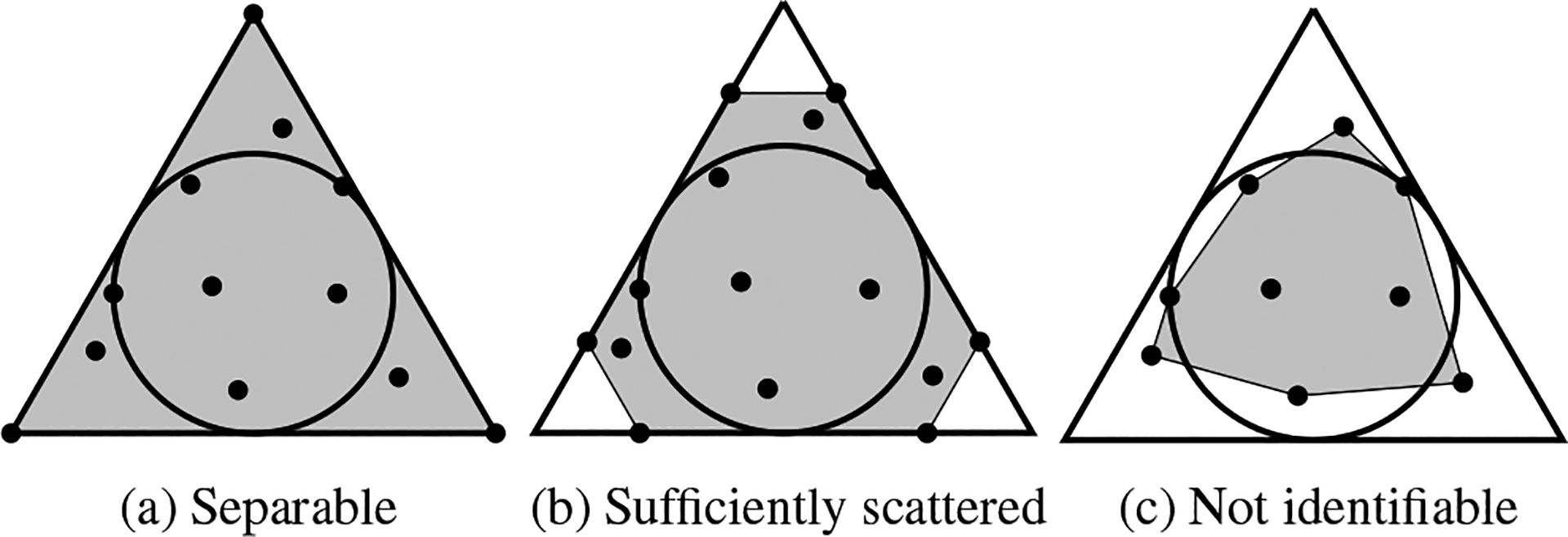
A geometric illustration of the sufficiently scattered condition (middle), a special case that is separable (left), and a case that is not identifiable (right). The triangle denotes the nonnegative orthant, the circle denotes the hyperbolic cone defined in Assumption 1, solid dots represent rows of , and the shaded regions represent cone .
One can also see from Figure 2a that the separability assumption, considered in [20] and in the context of NTD [13], is a very special case of sufficiently scattered. It requires that all the coordinate vectors be included in rows of , which makes cone , while the sufficiently scattered condition is allowed to grossly violate separability. In fact, it has been empirically observed that a nonnegative sparse matrix satisfies the sufficiently scattered condition with very high probability [18].
Our main result on the identifiability of NTD is presented as follows:
Theorem 1. Assume that , where all the ground-truth nonnegative Tucker factors are sufficiently scattered (Assumption 1). Let be an optimal solution of (4), then there exist permutation matrices and diagonal matrices such that
In other words, NTD is identifiable (Definition 1) if all the Tucker factors are sufficiently scattered.
Due to space limitation, the proof is relegated to the journal version.
2.2. Algorithm
In practice, the data tensor most likely does not admit an exact NTD . Therefore, when designing an algorithm for identifiability guaranteed NTD, one has to balance the identification criterion, the volumes of the Tucker factors in this case, and data fidelity. We propose to formulate the problem as
| (5) |
where is the regularization parameter that controls the balance between data fidelity and the identification criterion, and is the generalized Kullback-Leibler (GKL) divergence defined as
Ignoring terms that do not depend on the variables, and using the fact that columns of all sum to one, the GKL divergence is equivalent to (up to a constant difference)
| (6) |
where we overload the notation to denote summation over all elements of the tensor, denote element-wise multiplication, and the log of a tensor is also taken element-wise.
Since Problem 5 is non-convex, we propose to approximately solve it using successive convex approximation (SCA) [23]. At iteration when the updates are and , we define
Obviously and , which defines a probability mass function for each . Using Jensen’s inequality, we have that
which defines a convex and locally tight upperbound for the first term in the loss function of (5). Regarding the second term, we propose to simply take the linear approximation
where is the gradient of .
Now that we have derived a convex approximation to the objective of (5), which is separable down to each scalar variable, we can obtain the SCA updates without much difficulty. Due to space limitations, we skip some of the tedious steps and directly present the SCA algorithm as in (1). We would like to make two comments: 1) the operation performed in line 5 is mathematically represented as matrix multiplication of the -mode matricization of and the transpose of that of ; if the data tensor is large and sparse, this operation can be done efficiently via the TTMcTC (stands for tensor times matrix chain times core) kernel without instantiating the large and dense intermediate tensors [19]; and 2) the scalar in line 13 corresponds to the Lagrange multiplier of the constraint ; even though it is the solution of a nonlinear equation that cannot be solved analytically, it can be efficiently computed via bi-section.
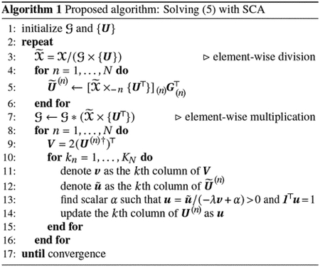
Regarding initialization, we propose to start by applying any algorithm for Tucker decomposition with orthonormal constraints, such as HOOI [5] or HOQRI [19], then apply the algorithm in [21] on each factor to obtain an initialization of ; the oblique rotations are then absorbed into the core tensor, followed by setting all negative values as zeros as initialization of .
3. NUMERICAL VALIDATION
We conclude the paper by providing some numerical validation to the proposed theoretical analysis. We focus on 3-way tensors of dimension and multilinear ranks . Since the focus of this paper is identifiability, we will synthetically generate the ground-truth Tucker factors and the core tensor , multiply them to get the data tensor , possibly contaminated with some noise. All the positive elements in the ground-truth factors are generated from independent exponential distributions. A portion of randomly selected elements in the ground-truth factors are set to zeros, since it has been observed that a sparse latent factor satisfies the sufficiently scattered condition with very high probability [18]. To resolve the scaling ambiguity, all columns of are rescaled to sum to one, leaving only permutation ambiguity to be resolved in the end.
In our first numerical experiment, we vary the level of sparsity of the latent factors and check how it affects identifiability. It has been shown in [16] that if a matrix is sufficiently scattered, then each columns of it contains at least zeros. This gives a rule-of-thumb of how sparse the latent factors should be in order to guarantee identifiability. Since we fix and , we could expect the model to be identifiable when the density, meaning the percentage of elements being nonzero, is lower than 90%. We vary the latent density from 50% to 95%, and check the probability of exact recovery. In each case, we generate 100 random instances of the ground-truth factors and the core tensor, multiply them to get the data tensor, and apply the initialization strategy of Algorithm 1. After resolving the permutation matrix via the Hungarian algorithm, we declare success if the estimation errors of all of the latent factors are less than 10−5. As we can see, the probability of success remains close to 1 even when the latent density is at the marginal 90%, but quickly goes to zero once it becomes higher.
Finally, we demonstrate the convergence behavior of the proposed Algorithm 1. In this case the data tensor is no longer noiseless. Since Algorithm 1 tries to solve Problem (5) with the generalized KL divergence, it makes sense to generate the elements of from independent Poisson distributions parameterized by the corresponding values in the Tucker product of the ground-truth factors. As we can see in Fig. 4, the algorithm does monotonically decrease the loss value. Due to the Poisson noise, the loss is not close to zero. However, as we will elaborate in the journal paper, the introduced volume-regularization still helps reduce the estimation errors of the latent factors.
Fig. 4:
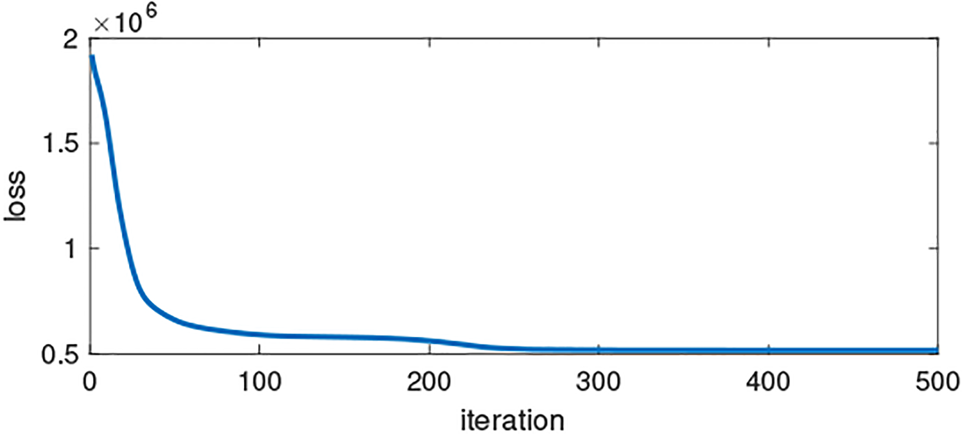
An instance of the convergence of Algorithm 1.
Fig. 3:
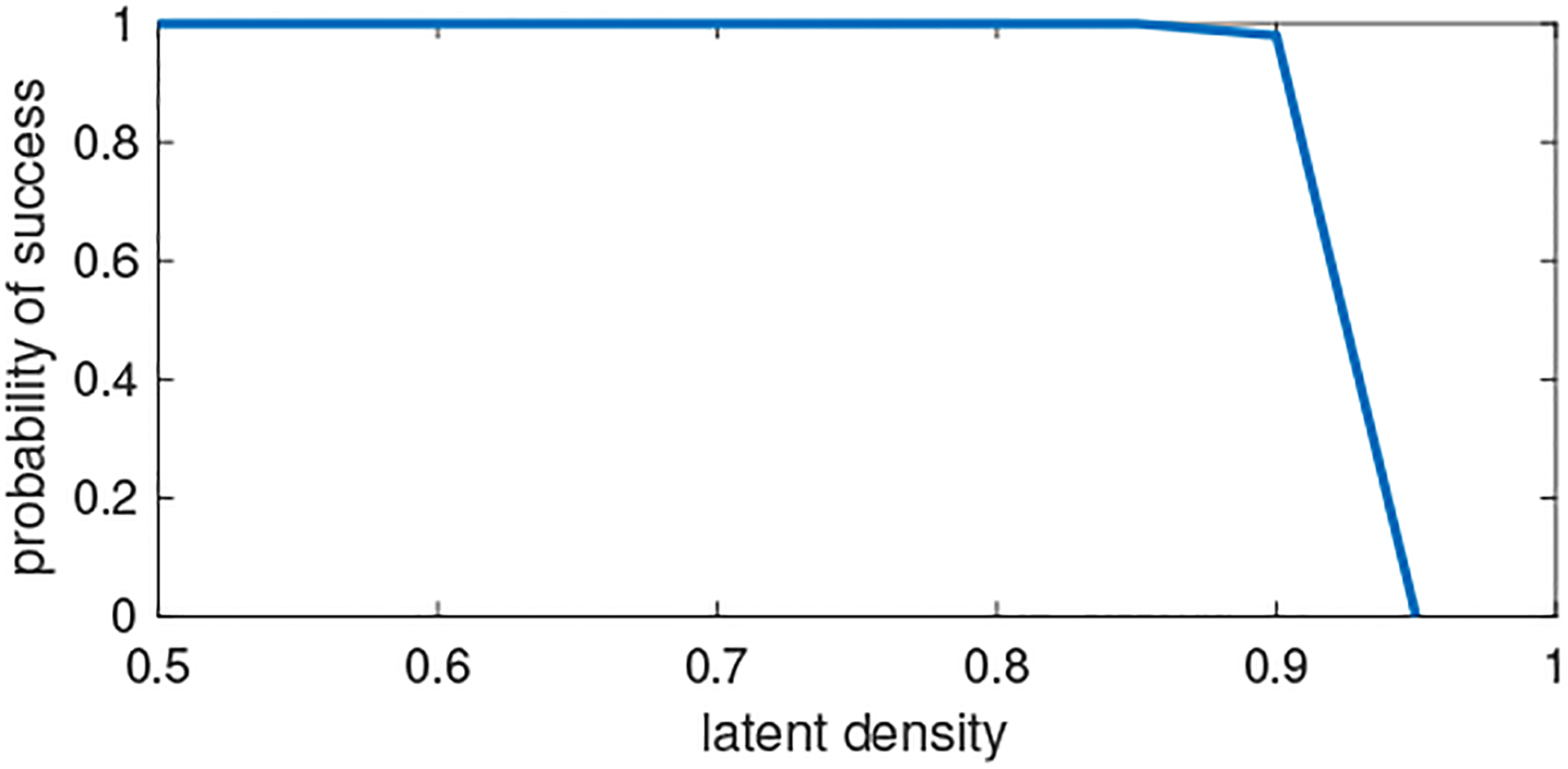
Probability of exact recovery of the latent factors as we vary the density of the latent factors.
Acknowledgments
Supported in part by NSF ECCS-2237640 and NIH R01LM014027.
REFERENCES
- [1].Kolda TG and Bader BW, “Tensor decompositions and applications,” SIAM Review, vol. 51, no. 3, pp. 455–500, 2009. [Google Scholar]
- [2].Sidiropoulos ND, De Lathauwer L, Fu X, Huang K, Papalexakis EE, and Faloutsos C, “Tensor decomposition for signal processing and machine learning,” IEEE Transactions on Signal Processing, vol. 65, no. 13, pp. 3551–3582, 2017. [Google Scholar]
- [3].Tucker LR, “Some mathematical notes on three-mode factor analysis,” Psychometrika, vol. 31, no. 3, pp. 279–311, 1966. [DOI] [PubMed] [Google Scholar]
- [4].De Lathauwer L, De Moor B, and Vandewalle J, “A multilinear singular value decomposition,” SIAM Journal on Matrix Analysis and Applications, vol. 21, no. 4, pp. 1253–1278, 2000. [Google Scholar]
- [5].—, “On the best rank-1 and rank-(R1,R2,…,RN ) approximation of higher-order tensors,” SIAM Journal on Matrix Analysis and Applications, vol. 21, no. 4, pp. 1324–1342, 2000. [Google Scholar]
- [6].Hitchcock FL, “The expression of a tensor or a polyadic as a sum of products,” Journal of Mathematics and Physics, vol. 6, no. 1–4, pp. 164–189, 1927. [Google Scholar]
- [7].Harshman RA, “Foundations of the PARAFAC procedure: Models and conditions for an” explanatory” multimodal factor analysis,” UCLA Working Papers Phonetics, vol. 16, pp. 1–84, 1970. [Google Scholar]
- [8].Kruskal JB, “Three-way arrays: rank and uniqueness of trilinear decompositions, with application to arithmetic complexity and statistics,” Linear algebra and its applications, vol. 18, no. 2, pp. 95–138, 1977. [Google Scholar]
- [9].Sidiropoulos ND and Bro R, “On the uniqueness of multilinear decomposition of N-way arrays,” Journal of Chemometrics: A Journal of the Chemometrics Society, vol. 14, no. 3, pp. 229–239, 2000. [Google Scholar]
- [10].Sidiropoulos ND, Bro R, and Giannakis GB, “Parallel factor analysis in sensor array processing,” IEEE transactions on Signal Processing, vol. 48, no. 8, pp. 2377–2388, 2000. [Google Scholar]
- [11].Lee DD and Seung HS, “Learning the parts of objects by nonnegative matrix factorization,” Nature, vol. 401, no. 6755, pp. 788–791, 1999. [DOI] [PubMed] [Google Scholar]
- [12].Kim Y-D and Choi S, “Nonnegative Tucker decomposition,” in 2007 IEEE conference on computer vision and pattern recognition. IEEE, 2007, pp. 1–8. [Google Scholar]
- [13].Zhou G, Cichocki A, Zhao Q, and Xie S, “Efficient nonnegative Tucker decompositions: Algorithms and uniqueness,” IEEE Transactions on Image Processing, vol. 24, no. 12, pp. 4990–5003, 2015. [DOI] [PubMed] [Google Scholar]
- [14].Xu Y, “Alternating proximal gradient method for sparse nonnegative Tucker decomposition,” Mathematical Programming Computation, vol. 7, no. 1, pp. 39–70, 2015. [Google Scholar]
- [15].Cohen JE, Comon P, and Gillis N, “Some theory on nonnegative Tucker decomposition,” in International Conference on Latent Variable Analysis and Signal Separation. Springer, 2017, pp. 152–161. [Google Scholar]
- [16].Huang K, Sidiropoulos ND, and Swami A, “Non-negative matrix factorization revisited: Uniqueness and algorithm for symmetric decomposition,” IEEE Transactions on Signal Processing, vol. 62, no. 1, pp. 211–224, 2013. [Google Scholar]
- [17].Fu X, Huang K, and Sidiropoulos ND, “On identifiability of nonnegative matrix factorization,” IEEE Signal Processing Letters, vol. 25, no. 3, pp. 328–332, 2018. [Google Scholar]
- [18].Fu X, Huang K, Sidiropoulos ND, and Ma W-K, “Nonnegative matrix factorization for signal and data analytics: Identifiability, algorithms, and applications,” IEEE Signal Processing Magazine, vol. 36, no. 2, pp. 59–80, 2019. [Google Scholar]
- [19].Sun Y and Huang K, “HOQRI: Higher-Order QR Iteration for Scalable Tucker Decomposition,” in ICASSP 2022–2022 IEEE International Conference on Acoustics, Speech and Signal Processing (ICASSP). IEEE, 2022, pp. 3648–3652. [DOI] [PMC free article] [PubMed] [Google Scholar]
- [20].Donoho D and Stodden V, “When does non-negative matrix factorization give a correct decomposition into parts?” Advances in neural information processing systems, vol. 16, 2003. [Google Scholar]
- [21].Huang K, Fu X, and Sidiropoulos ND, “Anchor-free correlated topic modeling: Identifiability and algorithm,” Advances in Neural Information Processing Systems, vol. 29, 2016. [Google Scholar]
- [22].Ben-Israel A, “A volume associated with m × n matrices,” Linear Algebra and Its Applications, vol. 167, pp. 87–111, 1992. [Google Scholar]
- [23].Razaviyayn M, Hong M, and Luo Z-Q, “A unified convergence analysis of block successive minimization methods for nonsmooth optimization,” SIAM Journal on Optimization, vol. 23, no. 2, pp. 1126–1153, 2013. [Google Scholar]


