

Abstract
Learning methods, such as conventional clustering and classification, have been applied in diagnosing diseases to categorize samples based on their features. Going beyond clustering samples, membership degrees represent to what degree each sample belongs to a cluster. Variation of membership degrees in each cluster provides information about the cluster as a whole and each sample individually which enables us to have insights toward precision medicine. Membership degrees are measured more accurately through removing restrictions from clustering samples. Bounded Fuzzy Possibilistic Method (BFPM) introduces a membership function that keeps the search space flexible to cluster samples with higher accuracy. The method evaluates samples for their movement from one cluster to another. This technique allows us to find critical samples in advance those with potential ability to belong to other clusters in the near future. BFPM was applied on metabolomics of individuals in a lung cancer case-control study. Metabolomics as proximal molecular signals to the actual disease processes may serve as strong biomarkers of current disease process. The goal is to know whether serum metabolites of healthy human can be differentiated from those with lung cancer. Using BFPM, some differences were observed, the pathology data were evaluated, and critical samples were recognized.
Keywords: Data type, Critical object, Bounded Fuzzy Possibilistic Method, Sample movement, Clustering, Membership function, Lung cancer, Pathology, Metabolomics
1. Introduction
In diagnosing diseases from -omic analysis, some learning methods have been utilized. Furey et al. (2000) proposed support vector machine (SVM) method to classify tissues based on gene expression samples [1]. Shen et al. (2009) discussed some clustering techniques mostly latent variable models to reduce data dimension [2] and identify subtypes of breast and lung cancer. Liu et al. (2005) applied supervised learning strategies using genetic algorithms and SVM method to reduce discriminant gene features and overcome the complexity of large scale microarrays data [3]. In addition to partitioning samples, membership functions allocate a degree (between zero to one) to each sample [4]. In some methods, partial assignments are not covered and samples with degree one from one cluster have zero degree in other clusters. In some other methods, samples with degrees less than 1 from one cluster can obtain partial membership degrees in other clusters depending on how far their degrees are from 1 [5]. To reduce the limitations of clustering procedures and sample analysis, Bounded Fuzzy Possibilistic Method (BFPM) [6] identifies membership degrees with respect to all clusters in contrary to methods that sharply separate samples. Using BFPM, we evaluate sample movement based on assigned membership degrees to predict the behavior. Studying membership degrees in addition to clustering provides better insights on samples and may lead to prevention and more effective treatments. Here, we apply BFPM on a set of samples featured by metabolites. Metabolomics is an emerging technology platform that has shown early success in identifying biomarkers and mechanisms of diseases [7], [8]. The hypothesis is whether we can differentiate serum metabolites of healthy individuals from those with lung cancer. Actually, we want to differentiate not only healthy vs. Lung Cancer, but also associate patterns with clinics-pathological behaviour of lung cancer. The rest of this paper is organized as follows. Some of the well known approaches in machine learning are explored in Section 2. Different data types in machine learning have been studied in Section 3. Several advanced research activities have been explored as related work in Section 4. A case study on metabolites is discussed in Section 5. Tissue and serum samples are compared in this section too. Future plans and discussions are studied in Section 6, and a brief conclusion is presented in Section 7.
2. An overview to clustering methods and membership functions
Clustering is a form of unsupervised learning methods that categorizes samples based on their similarities. Unlike supervised methods, there is no training step in clustering approaches [9], [10]. Assume a set of n samples presented as numerical feature-vector data in dimensional search space as categorized in clusters. Samples are assigned membership degrees represented as a matrix known as partition or membership matrix, where is the membership degree for the sample (object) in the cluster. The most common membership functions can be categorized as crisp, fuzzy, probability, possibilistic, and bounded fuzzy possibilistic methods.
2.1. Crisp methods
Crisp methods classify samples in non-empty and mutually disjoint subsets, presented by Eq. (1).
| (1) |
In these methods can obtain values either zero or one. means that the sample is a member of the cluster, and indicates that the sample does not belong to the cluster. Crisp methods are mostly used in some partitioning approaches such as hierarchical methods, SVM, decision trees, and network fusion methods where samples are sharply separated [11].
2.2. Fuzzy or probability methods
Fuzzy or probability methods, presented by Eq. (2), make the search space more flexible for samples to participate in more than one cluster by partial membership degrees [12].
| (2) |
Fuzzy methods have some limitations in membership assignments due to allowing each sample to be a member of only one cluster with full membership degree, shown by constraint () [13], [14].
2.3. Possibilistic methods
Possibilistic methods, presented by Eq. (3), provide wider environment for samples to participate in more clusters [15].
| (3) |
Possibilistic methods relax the membership condition () by () [16]. The method has some drawbacks in its early initializations [17]. These methods also lack of definite upper and lower boundaries for each cluster [18]. Without the definite boundaries, on one side, the method cannot be implemented precisely, and on the other side, samples participate in other clusters with less flexibility.
2.4. Bounded Fuzzy Possibilistic Method
Bounded fuzzy possibilistic method (BFPM), presented by Eq. (4), provides the most flexible environment for samples to participate in multiple clusters, and even obtain full membership degrees from all clusters.
| (4) |
BFPM covers crisp, partial, and full membership degrees for samples with respect to all clusters and allows them to obtain membership degrees from any cluster, with no limitation. Based on membership assignments and Eq. (1)-Eq. (4), it can be concluded:
As seen, each learning method makes use of a specific membership function in learning procedure. This study focuses on BFPM membership function as a superset of other membership functions to provide the most flexible searching space, besides assigning more precise membership degrees with respect to all clusters. In addition to membership function, there are other important parameters in learning methods which affect the accuracy of selected approaches. Similarity functions and data type can be also selected as crucial parameters in learning procedures [11], [19]. The most accurate similarity functions lead to extracting similar samples [20] with known or labelled samples which consequently result in distinguishing a proper category for specific samples [21], [22]. This paper leaves similarity functions untouched in following sections, but considers the data types by illustrating data type taxonomies and focusing on those that are applied in the case study.
3. Data Type
In learning methods, one of the most important factors is type of data. Lack of well consideration on data types misleads learning methods to recognize objects from the same category and eventually lose needed information. The first and the most important factor in learning methods is the ability to differentiate data objects in order to choose accurate approaches in learning procedures with respect to each particular object. Each type of object has its own properties and influences on final results, regardless of type of learning method. To differentiate data types and their impacts on learning approaches, analysing data types from different points of view is indispensable. This paper explores different types of objects with regard to their behaviour and their structures. Structural-based and behavioural-based categories are two main data type categories, and each one of the categories includes different subcategories, briefly explored as follows.
3.1. Structural-based Category
Data objects are categorized into different groups according to their structures listed as single or multivariable, complex, and advanced objects.
- Single or Multi-variable objects
- Single-variable object: Objects of a single variable can be presented by , where n is the number of objects ().
- Multi-variable object: Objects with more variables on data set or population , where n is the number of objects and presents each object with d variables or dimensions.
- Complex objects: Due to the growth of data in recent years, learning methods need to consider data objects in different structures rather than above mentioned categories. Data objects that are categorized as complex objects are listed as follow.
- Structured Data Object: HTML files.
- Semi-structured Data Object: XML files.
- Unstructured Data Object: text files.
- Spatial Data Objects: maps/medical images.
- Hypertext: messages, reports, documents,… .
- Multimedia: videos, audio, musics, and ….
- Advanced Objects: The need of evaluating data objects in an accurate and efficient way leads to considering a set of objects with common properties as a new object or a superset of some objects to accelerate the learning procedures. Advanced objects can be categorized as follow.
- Sequential Patterns.
- Graph and Sub-graph Patterns.
- Objects in Interconnected Networks.
- Data Stream, or Stream Data.
- Time Series.
3.2. Behavioural-based Category
In addition to the structure of data object, learning methods need to consider the behaviour of each data object individually in order to evaluate the influences of each particular object. According to model-based approaches, data objects are divided into different categories by attempting to optimize the fit between the data and some mathematical models, when the data objects are generated by a mixture of underlying probability distributions [23]. The data model can be extracted from a Gaussian mixture, a regression-based, or a proximity-based model. Data objects are categorized into three main categories with respect to their behaviour known as Normal, Outlier, and Critical objects [24].
Normal Objects Data object can be considered as normal object, if the object follows one of the discovered data patterns.
Outliers Data objects that do not fit the model of the data, and do not obey the discovered patterns of the data are considered as outliers [25]. Outliers are far from the rest of objects in data sets and may change the behaviour of the model if they are considered in learning procedures and measurements. Outliers are mostly known as noise or exceptions and are usually removed from data sets in most applications. There are however some applications that perform based on anomaly analysis while some statistical distributions and probability models are used to check the occurrence of outliers [26].
Critical Objects Unlike outliers, a data set may contain objects that follow the discovered patterns and do fit into more than one even all data models. The model and pattern of the data remain unchanged by considering critical objects, as these objects obey the patterns of the data and they are in the discovered patterns. Critical objects are mostly known as partial or full members of several clusters or partitions. Removing critical objects from data sets result in losing useful information, so these objects cannot be removed from any cluster that they participate in. The other important property of critical objects is that they have potential ability to move from one cluster to another (object’s movement) by getting small changes even in one dimension in feature spaces [27].
Further to the data type’s taxonomies, this paper provides some experimental verifications on multi-variant, normal and critical objects with regard to lung cancer samples. The idea is to evaluate the relations between different data types and some particular diseases. This paper also considers outliers in its experimental verifications without discussing about outlier detections.
4. Related Work
Sayes et al. (2007) gathered useful information related to feature selection techniques from machine learning and data mining to mention the importance of choosing the proper features in learning procedures [28]. Authors discussed about some approaches in different categories of features selections approaches known as Filter, Wrapper, and Embedded or Hybrid methods. Advantages and disadvantages of using any type of feature selection techniques have been explored by the authors. The discussion was mostly related to classification techniques where the learning methods have some background knowledge about the features in advance, and the knowledge helps the learning method to supervise the training strategy. The goal of the paper was to deal with the data sets that suffer the lack of enough samples or need to work on high dimensional search space [29]. The paper also evaluated the feature selection approaches according to structure of data objects either from uni-variant or multivariant category. Moving towards working with big data in high dimensional search space [30], the art of using feature selection for choosing the most important features to reduce the complexity and also obtaining the better accuracy is undeniable [31]. Zou et al. (2016) discussed about the pros and cons of filter and wrapper methods by studying the challenges of different methods on big data in dimensionality reduction from high to low dimensional search space [32]. The authors proposed a new distance function named Max-Relevance-Max-Distance based dimensionality reduction in their feature selection strategy in classification problems. Max-relevance-max-distance has been used in proteinprotein interaction prediction and image classification. One of the challenges in classification is identification of the border of each class. Using genome information as instrumental variables, Yazdani et al. (2016) have introduced an approach for the border identification based on effect size and directionality between variables [33], [34]. Unlike classification methods, clusterings make use of unsupervised methods. Xu et al. (2015) applied a clustering algorithm named shared nearest neighbor (SNN)-Cliq to cluster single-cell transcriptomes with regard to group cells that belong to the same cell types based on gene expression patterns [35]. The authors implemented their method using the most well-known Euclidean distance function to evaluate the neighbours and applied their method on human cancer and embryonic cells. Further to the authors, in single-cell transcriptome analysis, clustering helps to group individual cells based on their gene expression levels, which consequently lead to characterizing cell compositions in tissues to obtain better view on the physiology and pathology of the tissues and the developmental process. Lu et al. (2015) considered the causes of cancers by paying more attention to molecular abnormalities [36]. They followed the idea of personalized cancer therapy (PCT), by determining the exact alterations and molecular abnormalities of a specific cancer, where different types of cancer are caused by different genetic abnormalities (e.g., mutation, deletion, replication, translocation, and so on). The importance of using bioinformatics techniques in mathematical and computational systems in assessing genomic and molecular abnormalities has been covered by the authors. Kunz et al. (2017) considered lung cancer as a late diagnosis and limited intervention treatment, which bioinformatics can contribute to the development of non-invasive diagnostic tools for early lung cancer diagnosis [37]. They explored several bioinformatics methods and tools on microRNAs and non-coding RNAs. The authors explored different pathologic types of Non-Small Cancer Cell (NSCC) adenocarcinoma (AC) and squamous cell carcinoma (SQ) as 85% of the most often diagnosed subtype, whereas small-cell lung carcinoma (SCLC) as 15%) of the most aggressive subtype but less observed, in addition to list several tools for different proposes in genome browser, Folding prediction, Functional classification, Functional analysis, Interactions/pathways, Promotor analysis, nRNA sequence database, and so on.
5. Methodology
Extracting knowledge from datasets can be obtained by running different learning methods, either supervised (classification) or unsupervised (clustering) methods. The accuracy of classification techniques is mostly measured through the percentage of the correct labelled samples and strongly depends on the correct selection of samples and the number of samples in each class [38]. A large number of samples in one class dominates the accuracy and using some techniques such as t-test are needed to control the quality for the small sizes [38]. Therefore, in this study, we aim to utilize clustering techniques due to the different number of case and control individuals in our dataset. Furthermore, clustering techniques can lead to presenting the degree that cases are different from controls. We here employ BFPM clustering method to illustrate the similarity between samples. Moreover, covering sample movements and having a flexible search space encouraged us to present Algorithm 1 [5] in clustering methods based on BFPM membership function. The former concept leads to computing the potential ability of each sample to participate in another cluster, and the latter one is to cluster samples based on a flexible search space (diversity). Using BFPM, facilitates finding critical samples those that are about to move from healthy to cancer category or vice versa.
5.1. BFPM Algorithm
BFPM algorithm is introduced to assess the behaviour of healthy, cancer, and critical samples in addition to provide a flexible clustering search space. The algorithm aims to reveal information about healthy and lung cancer samples through analysing metabolites.
| Algorithm 1 BFPM Algorithm | |
|---|---|
|
|
Eq. (5) shows how the algorithm calculates based on a distance function, here Euclidean distance. Eq. (6) describes how the prototypes will be updated in each iteration using BFPM membership function presented by Eq. (4). The algorithm runs until reaching the condition:
The value assigned to is a predetermined constant that varies based on type of samples and clustering problems. is the () partition matrix, is the set of cluster centres (prototypes) in , is the fuzzification constant to provide different distance measurements, and is any inner product A-induced norm. Different values of provide different distance functions in different norms. In the proposed algorithm the Euclidean distance function, which is presented by Eq. (7), is utilized as a similarity function in membership assignments.
| (7) |
where is the number of features or dimensions, and and are two different samples in dimensional search space.
5.2. Case Study
Metabolomics is emerging as an important technology platform that measures chemistry which represents an integrated readout of upstream genetic, transcriptomic, and proteomic variation [39], [40]. In a case and control lung cancer study, we want to know if there is any difference between serum metabolites of case and control. We also want to evaluate the pathology data through tissue metabolites.
Study Sample:
Serum and tissue samples were obtained from the Harvard/MGH lung cancer susceptibility study repository. Informed consent was obtained from lung cancer patients and healthy controls prior to banking samples and after the nature and possible consequences of the study were explained. There are 231 samples, 101 are tissue samples and 101 are serum samples of the same individuals with lung cancer and 29 are serum samples of healthy individuals. In total, 61 metabolites (spectral regions) were measured in the following process. Researchers were blinded to the status of the samples during all measurement and experimental steps. Samples were stored at −80° C until to analysis. High resolution magic angle spinning magnetic resonance spectroscopy (HRMAS MRS) measurements were performed using our previously developed method on a Bruker Avance (Billerica, MA) 600 MHz spectrometer. Measurements were conducted at 4° C with a spin-rate of 3.6 Hz and a Carr-Purcell-Meiboom-Gill sequence with and without water suppression. Ten μL of serum or ten μg of tissue were placed in a 4 mm Kel — F zirconia rotor with ten μL of D2O added for field locking. HRMAS MRS spectra were processed using AcornNMR-Nuts (Livermore, CA), and peak intensities from 4.5 — 0.5 ppm were curve fit. Relative intensity values were obtained by normalizing peak intensities by the total intensity of the water unsuppressed file. The resulting values which were less than 1% of the median of the entire set of curve fit values were considered as noise and eliminated. Spectral regions were defined by regions where 90% or more of samples had a detectable value, with 32 regions resulting. Following MRS measurement, tissues were formalin-fixed and paraffin-embedded. Serial sectioning was performed by cutting 5μm — thick slices at 100μm intervals throughout the tissue, resulting in 10 — 15 slides per piece. After haemotoxylin and eosin (H&E) staining, a pathologist with > 25 years experience read the slides to the closest 10% for percentages of the following pathological features: cancer, inflammation/fibrosis, necrosis, and cartilage/normal. The available dataset is normalized in an interval [0, 1] which includes 71 features in total. Features contain five categorical or qualitative variables and all of them are nominal, 61 independent numerical or quantitative variables (metabolites) which all of them are ratio with discrete values, and five numerical variables as ratio type with discrete values. Feature selection techniques also assist the learner to obtain better accuracy, in addition to reduce the complexity of the procedure [41], but in here, the features are considered with the same priority and all the features are evaluated in the clustering procedure.
5.2.1. Clustering and analysing serum samples
Here, we utilized the BFPM for clustering to see behavior of samples tested based on metabolites. The BFPM employs membership degrees for clustering samples and provides information about each sample individually in addition to insights into reliability of the clusters. In general, the number of clusters can be estimated using different techniques, such as visualization of the dataset, optimization under probabilistic mixture-model framework, using certain validity indices to evaluate the intra-cluster and inter-cluster similarities, and other heuristic approaches [42]. However, each of these approaches suffers some sort of bias. For example, validity indices can be biased through using some parameters in the evaluation’s procedures such as dominant feature in similarity functions [43]. Visualization techniques on the other hand are extremely sensitive to the chosen dimensions [44], [45]. In this study however, we analyze the results obtained from different number of clusters to find patterns in the data associated with clinic-pathological behavior of lung cancer to differentiate healthy from lung cancer samples.
Some results of clustering are depicted in Fig. 1 and Fig. 2 where on the axes, samples are located. The first 101 samples are serum metabolites of individuals with lung cancer. The last 29 samples are serum metabolites of the healthy individuals. On the axes membership degrees for each sample is provided, varying from 0 to 1. Fig. 1.b shows two lines. The upper one connects the membership degrees of each sample in the current cluster in Fig. 1.a. The lower line connects membership degrees of each sample in the second cluster. Here, we analyze the serum samples excluding the tissue samples with the aim of highlighting similarities and differences among the serum samples. By analysing serum samples with regard to both clusters, Fig. 1, we see healthy and cancer samples spread in both clusters. This is not surprising due to sharing common parameters between cancer and healthy samples. Extracting similarity between healthy and unhealthy individuals through serum samples was a lead to increase the number of clusters to check in what extend samples show their properties. Therefore, different number of clusters have been chosen and interesting information has been obtained accordingly. The most significant achievements were related to the results of clustering samples into four clusters, presented by Fig. 2. Digging in Fig. 2, we could observe differences between healthy and cancer samples, reviewed below. Very interestingly, we noticed that no healthy sample is categorized in the diamond cluster. We can also see samples in the diamond cluster have high membership degrees that represent the reliability of the cluster. Having no healthy sample in the diamond cluster generates a hypothesis that these samples must differ from the other cancer samples. Results from analyzing covariates of individuals in the diamond cluster and comparing with the rest of cancer individuals are summarized in Table 1. These individuals have shorter survival time and nearly 15% more with squamous cell carcinoma than adenocarcinoma.
Fig. 1.
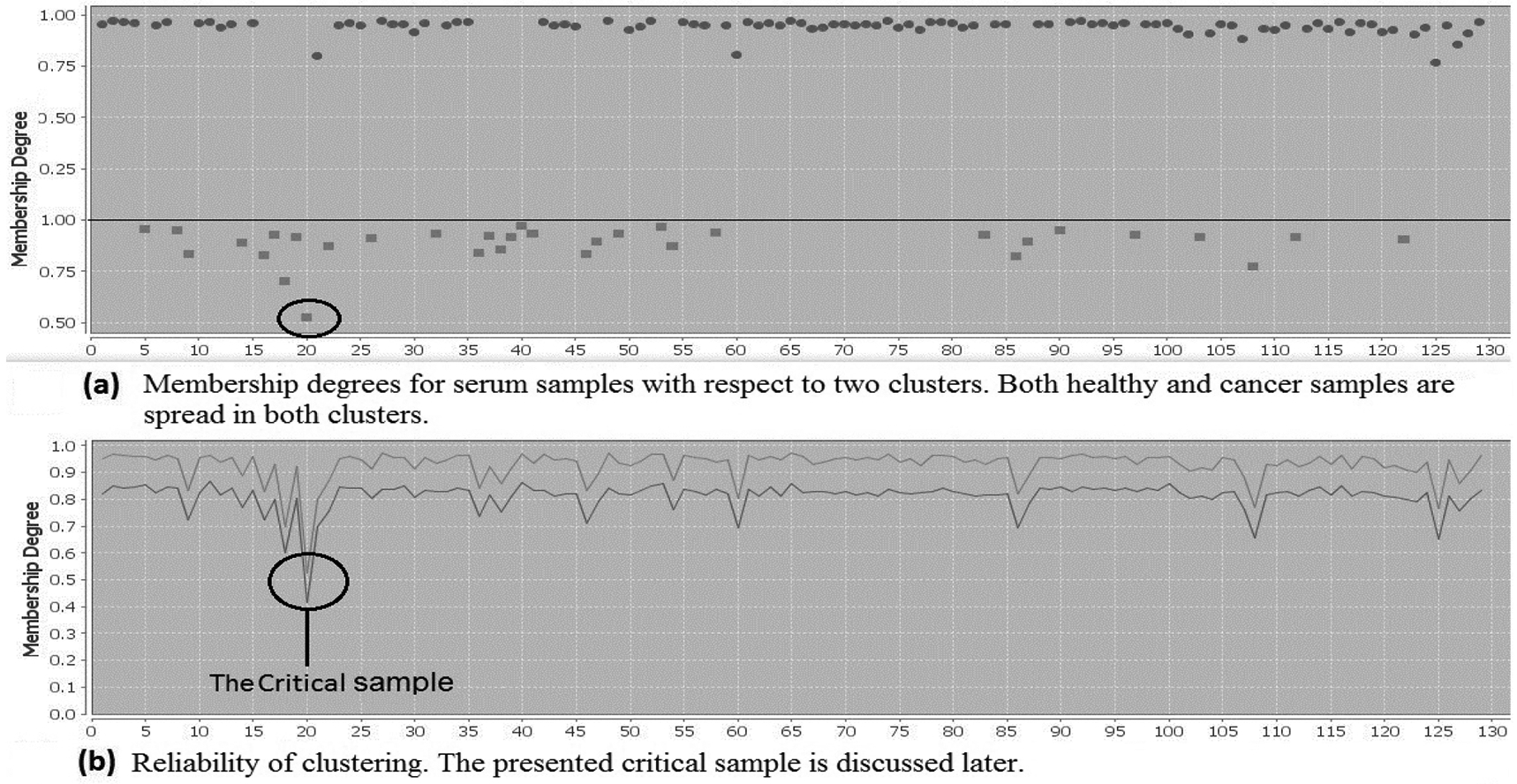
serum samples tested by 61 metabolites using BFPM. The first 101 samples on X axis are from serum of individuals with lung cancer, and the last 29 samples are from healthy individuals. The Y axis represents the membership degrees in an interval [0, 1].
Fig. 2.
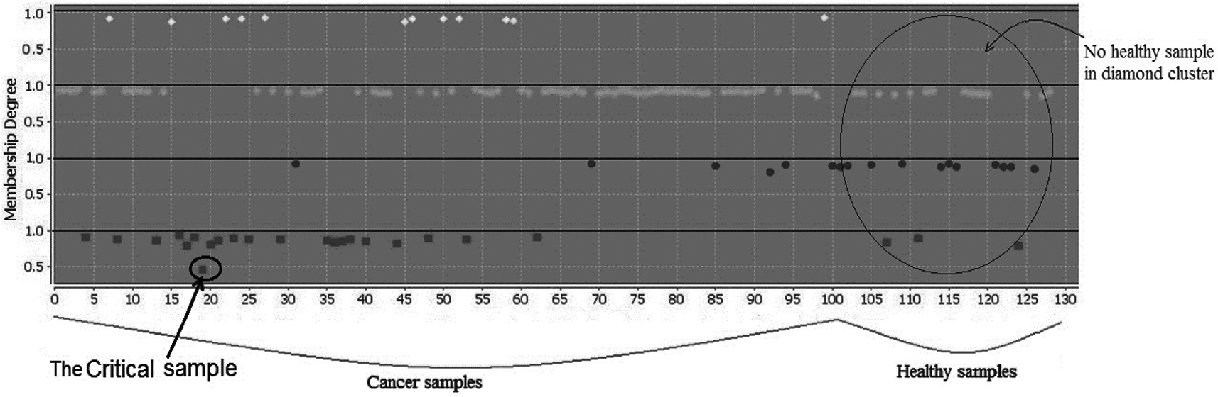
Serum samples in 4 clusters. No healthy sample in the diamond cluster generates a hypothesis that diamond samples are different from the other cancer samples. This hypothesis is strengthened through the covariate assessment.
TABLE 1.
Comparison of the diamond samples and the rest of cancer samples with regard to the covariant variables: five year survival (short/long), cancer stage (low/high), average age, and cancer type (squamous (s) / adenocarcinoma (a)).
| Serum metabolites | Samples No. | Survival(s) | Survival(l) | Stage(l) | Stage(h) | Ave. age | Type(s) | Type(a) |
|---|---|---|---|---|---|---|---|---|
| Diamond samples | 12 | 63.30 % | 36.70 % | 83.33 % | 16.67 % | 64.82 | 57.33 % | 42.67 % |
| Cancer samples excluding diamond | 89 | 59.09 % | 40.91 % | 58.43 % | 41.57 % | 66.08 | 44.94 % | 55.06 % |
| Normal samples | 29 | - | - | - | - | 66.83 | - | - |
Very similar to the diamond cluster that includes no healthy individuals, the square cluster includes only three healthy individuals and the rest of 23 individuals have cancer. Table 2 includes the analysis of individuals in the square cluster in terms of covariates. From Table 1 (analysis of cancer samples in the diamond cluster) and Table 2 (analysis of cancer samples in the square cluster), we see percentages of cancer types adenocarcinoma and squamous cell carcinoma are different in these two clusters. We may conclude that the serum metabolites of individuals with adenocarcinoma cancer is different from squamous cell carcinoma cancer and they are different from healthy metabolites. This means not only some differences between the serum metabolites of healthy and cancer individuals are observed but also the serum metabolites of different types of cancers are different. On the other hand, only six out of 101 cancer samples are categorized in the circle cluster where more than one third of the healthy samples are categorized. This generates a hypothesis that these six cancer samples have distinctive features from other cancer samples. Table 3 compares the circle samples with the remaining cancer samples. We can see these six individuals are almost 8 years younger than the rest of cancer samples and more than 66% are adenocarcinoma patients. They are almost 11 years younger than the healthy samples in the same cluster. We may conclude younger people with lung cancer have metabolites similar to older healthy people.
TABLE 2.
Analysing the square samples with regard to the covariant variables: five year survival (short/long), cancer stage (low/high), average age, smocked cigarette, and cancer type (squamous (s) / adenocarcinoma (a)).
| Serum metabolites | Samples No. | Survival(s) | Survival(l) | Stage(l) | Stage(h) | Ave. age | Pk. of cig. | Type(s) | Type(a) |
|---|---|---|---|---|---|---|---|---|---|
| Cancer samples in square cluster | 21 | 40.91 % | 59.09 % | 60.87 % | 39.13 % | 65.31 | 65.72 | 39.13 % | 60.87 % |
| Cancer samples excluding squares | 80 | 61.25 % | 38.75 % | 59.75 % | 41.25 % | 65.48 | 56.44 | 46.25 % | 53.75 % |
| All cancer samples | 1 01 | 60.40 % | 39.60 % | 61.39 % | 38.61 % | 65.93 | 60.43 | 46.53 % | 53.47 % |
| Normal samples in square cluster | 3 | - | - | - | - | 74.60 | 48.71 | - | - |
TABLE 3.
Circle cluster. Analysis of samples in the circle cluster shows that cancer individuals in this cluster are obviously younger that the healthy individuals in this cluster.
| Serum metabolites | Samples No. | Survival(s) | Survival(l) | Stage(l) | Stage(h) | Ave. age | Type(s) | Type(a) |
|---|---|---|---|---|---|---|---|---|
| Cancer samples in circle cluster | 6 | 50.00 % | 50.00 % | 66.66 % | 33.34 % | 58.60 | 33.34 % | 66.66 % |
| Healthy samples in circle cluster | 11 | - | - | - | - | 64.65 | - | - |
| Healthy samples in circle without outliers | 9 | 69.35 | ||||||
| Cancer samples excluding circle | 95 | 61.05 % | 38.95 % | 61.05 % | 38.95 % | 66.39 | 47.37 % | 52.63 % |
| Cancer samples | 101 | 60.40 % | 39.60 % | 61.39 % | 38.61 % | 65.93 | 46.53 % | 53.47 % |
5.2.2. Critical Samples
According to the properties of data types, critical samples follow the patterns of more than one cluster fully or partially. Therefore, critical samples obtain membership degrees from more than one cluster [27]. As a result, they are distinguishably separated from the other samples in a cluster according to their behaviour with respect to both clusters, see Fig. 1.b for a critical sample indicated by a black circle. Fig. 1.b shows that the critical sample obtained very similar membership degrees in both clusters in comparison with the other serum samples. In Table 4, we compare the critical sample with the other cancer samples in the same (square) cluster. In the analysis, we noticed that one sample, number 20 in Fig. 1.b, obtained almost similar membership degrees from both clusters. It has distinguishably a lower membership degree compared to the other samples in the cluster, Fig. 2.a. Critical objects can be chosen with a predefined threshold that varies by approaches and datasets. The threshold can be calculated based on the lower boundary of the assigned membership degrees to object with respect to all clusters [6]. The critical object presented here is selected as an example. The advantage is to know how to evaluate and treat those samples with potential ability to move from healthy to unhealthy cluster or vice-versa.
TABLE 4.
The critical sample. Information for the critical sample and the other samples in the same (square) cluster.
| Serum metabolites | Samples No. | Survival(s) | Survival(l) | Stage(l) | Stage(h) | Ave. age | Type(s) | Type(a) |
|---|---|---|---|---|---|---|---|---|
| The critical sample | 1 | + | − | + | − | 71.60 | + | − |
| Cancer samples in square cluster | 21 | 40.00 % | 60.00 % | 61.91 % | 38.09 % | 65.31 | 42.86 % | 57.14 % |
| Cancer samples excluding the critical sample | 20 | 36.84 % | 63.16 % | 60.00 % | 40.00 % | 64.99 | 40.00 % | 60.00 % |
| All cancer samples | 101 | 60.40 % | 39.60 % | 61.39 % | 38.61 % | 65.93 | 46.53 % | 53.47 % |
5.2.3. Pathology data assessment
The BFPM clustering approach was used on the metabolomic case and control data set to evaluate dissimilarity between healthy and cancer samples according to the stage of their diseases. Through categorizing the serum samples in four clusters in Fig. 2, using BFPM, we found that the diamond cluster includes only the cancer samples and not healthy sample. Through further analyses of these samples and comparing with the rest of cancer samples with regard to covariates, we noticed that the diamond samples have severe cancer, shorter survival time, shorter life time, and more squamous cell carcinoma rather than adeno carcinoma cancer. It should be noted that the results presented in Table 5 to Table 8 are related to the 101 tissue samples matched with the 101 serum samples. From the analysis of the pathology data depicted in Table 5, we observed that the diamond samples have more than 7% cancer cell as compared with the other cancer samples. However, in terms of necrosis cells, the diamond samples have 50% necrosis cells less than other samples. In Table 6 and Table 7, we also analyzed the pathology data of the diamond samples. From Table 6, we see almost 86% of the diamond samples with short survival time are diagnosed at the stage low and almost 60% have short survival time while through pathology they have less than 20% cancer cell. From Table 7, we see more than 45% of the diamond samples have less than 10% necrosis while their survival is short. Therefore, from Tables 6 and 7, we may conclude that the diamond samples are misdiagnosed through pathology analysis. However, from serum analysis, the diamond samples with severe cancer are separated from healthy individuals. In Table 8, we look at the pathology of the critical sample. We can see that 100% cells of the sample are benign and therefore, the sample is diagnosed at stage low, while the survival time of the critical sample is low. Table 9 provides some information related to the star samples, cancer and healthy samples in star, presented by Fig. 2 according to covariant variables: five year survival (short/long), cancer stage (low/high), average age, smoked cigarette, and cancer type (s/a).
TABLE 5.
Pathology data analysis. A comparison between the pathology data of the diamond samples from Fig. 2 and the rest of cancer samples. The diamond samples have more cancer cells and less than 50% necrosis cells as compared with the rest of the cancer samples. Note that the diamond samples are found with sever cancer through the serum analysis.
| Tissue metabolites | Cancer % | Necrosis % | Necrosis =0 | Necrosis > 10% | Necrosis > 25% | Necrosis > 50% | Benign % |
|---|---|---|---|---|---|---|---|
| Diamond samples | 26.47 % | 6.56 % | 66.67 % | 16.67 % | 8.33 % | 0.00 % | 66.97 % |
| Tissue samples excluding diamond | 19.17 % | 12.52 % | 66.34 % | 22.78 % | 14.85 % | 9.90 % | 67.32 % |
TABLE 8.
The pathology data of the critical sample and comparison with its cluster, square, and the rest of samples.
| Serum metabolites | Cancer % | Necrosis % | Necrosis =0 | Necrosis > 10% | Necrosis > 25% | Necrosis > 50% | Benign % |
|---|---|---|---|---|---|---|---|
| The critical sample in square cluster | 0.00 % | 0.00 % | - | - | - | - | 100.00 % |
| Tissue samples in square cluster | 7.33 % | 14.69 % | 65.57 % | 17.40 % | 17.40 % | 13.04 % | 73.45 % |
| Tissue samples | 19.17 % | 12.52 % | 66.34 % | 22.78 % | 14.85 % | 9.90 % | 67.32 % |
TABLE 6.
Analyzing the diamond samples through their pathology data. Almost 86% of the diamond samples with short survival time are diagnosed at stage low and almost 60% have short survival time while through pathology they have less than 20% cancer cell.
| Tissue cells | Survival(s)-stage(l) | survival(s)-benign(> 85%) | survival(s)-cancer(< 20%) | Survival(s)-cancer(< 50%) |
|---|---|---|---|---|
| Diamond samples | 85.79 % | 42.86 % | 57.14 % | 71.43 % |
TABLE 7.
Analysing the diamond samples through necrosis cells from the pathology data. More than 45% of the diamond samples have less than 10% necrosis while their survival is short.
| Tissue cells | Survival(s)-Necr.(=0%) | Survival(s)-Necr.( ≤ 10%) | Survival(s)-Necr.(≤ 25%) | Survival(s)-Necr.(≤ 50%) |
|---|---|---|---|---|
| Diamond samples | 36.36 % | 45.45 % | 54.55 % | 63.63 % |
TABLE 9.
Analyzing the star samples through their pathology data with regard to the covariant variables: five year survival (short/long), cancer stage (low/high), average age, smocked cigarette, and cancer type (squamous (s) / adenocarcinoma (a)).
| Serum metabolites | Samples No. | Survival(s) | Survival(l) | Stage(l) | Stage(h) | Ave. age | Pk. of cig. | Type(s) | Type(a) |
|---|---|---|---|---|---|---|---|---|---|
| Star samples | 77 | - | - | - | - | 66.72 | 54.58 | - | - |
| Cancer samples in star cluster | 62 | 58.02 % | 41.98 % | 59.68 % | 40.32 % | 66.01 | 57.29 | 51.61 % | 48.39 % |
| Healthy samples in star cluster | 15 | - | - | - | - | 69.45 | 43.35 | - | - |
6. Discussion
Bounded Fuzzy Possibilistic Method (BFPM) is a methodology to assign memberships to objects which can be used in clustering algorithms. Using BFPM, we clustered case and control samples tested by serum metabolites. BFPM can be applied on any dataset, as long as they are selected from or converted to the data types discussed above (single or multivariable, complex, and advanced objects). There are several parameters that lead to different results in clustering algorithms and membership function is considered as one of the most important parameters [6]. Clustering methods discussed in this paper utilize membership assignments in a way that prevents samples to easily participate in different clusters as a full or partial member [24]. However, BFPM due to its feature of membership assignments (), allows samples to participate in other, even all, clusters with a full or partial membership [5]. Through analysis of healthy and cancer individuals at different clusters, we generated some hypotheses. We tried to assess the hypotheses through analysis of covariates. In general, the number of clusters is estimated using different techniques with pros and cons, discussed in previous sections, but in this study we identify the number of clusters through analyzing the results. We noticed no healthy individual was in the diamond cluster. Therefore, we hypothesized that diamonds are different from the other cancer samples. This hypothesis was strengthened through comparison of the diamonds’ covariates and the rest. We also analyzed pathology data. Based on our analysis, the tissue samples could not be well clustered. We could also see the diamond samples hypothesized with sever cancer through serum metabolite had more than 7% cancer cell as compared with other cancer samples. However, in terms of necrosis cells, the diamond samples had 50% less necrosis cells than other samples. This paper discussed critical samples those that follow the patterns of more than one cluster. Knowing the type of samples and their potential movements in advance empowers us to cut the extra cost for further treatments. The proposed method recognizes critical samples, where most of conventional methods have difficulties in their membership assignments to analyze critical samples. Most of conventional distance functions (such as Euclidean distance) evaluate samples based on their total distance values. New similarity functions, which we introduced previously [43] provides an opportunity to work on each metabolite (feature) accordingly. Working on the impact of each metabolite on the final results using the proposed similarity functions is considered for a future plan. Analyzing the behavior of samples with respect to metabolites in supervised learning methods is also our future plan.
7. Conclusion
Bounded Fuzzy Possibilistic Methods (BFPM) provides an opportunity to identify some differences between serum of healthy and lung cancer samples. Using BFPM, we can also evaluate the pathology. The method recognizes the critical samples in prevention strategies for those samples that are going to move to another cluster. Our findings strengthened the hypothesis that there are some differences between serum metabolites of healthy and cancer samples.
Acknowledgement
Thanks go to Akram Yazdani, Alexander Davis, and Ahmad Samiei for their constructive comments. The work of providing data was supported by Grants R01CA115746, R21CA162959, and U01CA209414.
Biographies

Hossein Yazdani is a Ph.D. candidate at Wroclaw University of Science and Technology in Poland. He was a DBA, Network Manager, System Analyst in SADAD Informatics Corp. a subsidiary of MELLI Bank of IRAN. Currently, he cooperates with the Department of Information Systems, Faculty of Computer Science and Management, and Faculty of Electronics at Wrocaw University of Science and Technology. His research interests include BFPM, Critical objects, Dominant features, Machine learning, Distributed networks, Clustering, Network security, Bioinformatics, and Multi-objective optimization.

Leo L. Cheng, Ph.D., is an Associate Biophysicist, Pathology and Radiology at Massachusetts General Hospital and an Associate Professor of Radiology at Harvard Medical School. The USA National Cancer Institute sponsors his research. The research of his lab focuses on human prostate cancer, breast cancer, and lung cancer. His investigations on human malignancies work on the interface between Pathology and Radiology and attempt to establish alternative pathological procedures based on the current radiological technologies in general, and magnetic resonance spectroscopy and imaging techniques in particular.

David C. Christiani, is a professor, physician at Massachusetts General Hospital and Harvard Medical school. He is the leader of lung cancer program at Harvard cancer center. Dr. Christiani’s major research focus is Molecular Epidemiology of cancer. At MGH and HSPH he has led studies of genetic susceptibility to lung cancer as well as esophageal cancer. Recently, his work has expanded to the pharmacogenomics of treatment outcomes in lung and esophageal malignancies. He is investigating biologic markers of PAH and arsenic exposure for population studies. He also collaborates with international scientists on the molecular epidemiology of arsenic-induced bladder and skin cancer, and petrochemical exposures and brain neoplasms and leukemia in children.

Aazam Yazdani, Ph.D., M.Sc., is trained in statistical causal inference at mathematic and economic departments at Cambridge University, England and Friedrich Schiller University Jena, Germany. Since last 5 years, she has been working on developing algorithms and models to approach modern biomedical challenges. She has analyzed multiple biomedical datasets systematically. Her research is recognized at the 2015 Atlantic Causal Inference Conference at the University of Pennsylvania and some of her novel findings have already been validated.
Contributor Information
Hossein Yazdani, Department of Information Systems, Wroclaw University of Science and Technology, Poland..
Leo Cheng, Department of Pathology and Radiology, The University of Harvard, Medical School, Massachusetts, USA..
David C. Christiani, Department of Medicine, Massachusetts General Hospital/Harvard Medical School and Department of Environmental Health, Harvard T.H. Chan School of Public Health, Boston, MA. 02115, USA.
Azam Yazdani, Health Science center, University of Texas, USA and Climax Data Pattern, Inc..
References
- [1].Furey ST, Cristianini N, Duffy N, Bednarski DW, Schummer M, Haussler D, Support vector machine classification of cancer tissue samples using microarray expression data, Bioinformatics, 16(10), pp. 906–914, 2000. [DOI] [PubMed] [Google Scholar]
- [2].Shen R, Olshen AB, Ladanyi M, Integrative clustering of multiple genomic data types using a joint latent variable model with application to breast and lung cancer subtype analysis, Bioinformatics, 25(22), pp. 2906–2912, 2009. [DOI] [PMC free article] [PubMed] [Google Scholar]
- [3].Liu JJ, Cutler G, Li W, Pan Z, Peng S, Hoey T, Chen L, Ling XB, Multiclass cancer classification and biomarker discovery using GA-based algorithms, Bioinformatics, 21(11), pp. 2691–2697, 2005. [DOI] [PubMed] [Google Scholar]
- [4].Havens TC, Bezdek JC, Leckie C, Hall LO, Palaniswami M, Fuzzy c-means algorithms for very large data, IEEE, Transactions on Fuzzy Information and Engineering, 20(6), pp. 1130–1146, 2012. [Google Scholar]
- [5].Yazdani H, Fuzzy possibilistic on different search spaces, IEEE, International Symposium on Computational Intelligence and Informatics, pp. 283–288, 2016. [Google Scholar]
- [6].Yazdani H, Ortiz-Arroyo D, Choros K, Kwasnicka H, Applying bounded fuzzy possibilistic method on critical objects, IEEE, International Symposium on Computational Intelligence and Informatics, pp. 271–276, 2016. [Google Scholar]
- [7].Yazdani A, Bowman T, Marotta F, Cooke JP, Samiei A, Arachidonic acid as a target for treating hypertriglyceridemia reproduced by a causal network analysis and an intervention study, Metabolomics, 14(6), pp. 78, 2018. [DOI] [PubMed] [Google Scholar]
- [8].Yazdani A, Yazdani A, Liu X, Boerwinkle E, Identification of rare variants on metabolites in the pathway of carnitine for whole genome sequencing data analysis, Genetic Epidemiology, 40(6), pp. 486–491, 2016. [DOI] [PMC free article] [PubMed] [Google Scholar]
- [9].Barni M, Cappellini V, Mecoccie A, Comments on “A possibilistic approach to clustering”, IEEE, Transaction on Fuzzy Systems, 4(3), pp. 393–396, 1996. [Google Scholar]
- [10].Campello RJGB, A fuzzy extension of the Rand index and other related indexes for clustering and classification assessment, Pattern Recognition Letters, 28(7), pp. 833–841, 2007. [Google Scholar]
- [11].Tan PN, Steinbach M, Kumar V, Introduction to data mining, Pearson Addison Wesley, 2014. [Google Scholar]
- [12].Zadeh LA, Toward extended fuzzy logic - a first step, Elsevier, Fuzzy Sets and Systems, 160(21), pp. 3175–3181, 2009. [Google Scholar]
- [13].Pal NR, Pal K, Keller JM, Bezdek JC, A possibilistic fuzzy c-means clustering algorithm, IEEE, Transactions on Fuzzy Systems, 13(4), pp. 517–530, 2005. [Google Scholar]
- [14].Silva Filho TM, Pimentel BA, Souza RM, Oliveira AL, Hybrid methods for fuzzy clustering based on fuzzy c-means and improved particle swarm optimization, Expert Systems with Applications, 42(17), pp. 6315–6328, 2015. [Google Scholar]
- [15].Havens TC, Chitta R, Jain AK, Jin R, Speed-up of fuzzy and possibilistic kernel c-means for large-scale clustering, IEEE, International Conference on Fuzzy Systems, pp. 463–470, 2011. [Google Scholar]
- [16].Krishnapuram R, Keller JM, A possibilistic approach to clustering, IEEE, Transactions on Fuzzy System, 1(2), pp. 98–110, 1993. [Google Scholar]
- [17].Xenaki SD, Koutroumbas KD, Rontogiannis AA, A novel adaptive possibilistic clustering algorithm, IEEE, Transactions on Fuzzy Systems, 24(4), pp. 791–810, 2016. [Google Scholar]
- [18].Yang MS, Lai CY, A robust automatic merging possibilistic clustering method, IEEE, Transactions on Fuzzy Systems, 19(1), pp. 26–41, 2011. [Google Scholar]
- [19].Weller-Fahy DJ, Borghetti BJ, Sodemann AA, A survey of distance and similarity measures used within network intrusion anomaly detection, IEEE, Communication Surveys and Tutorials, 17(1), pp. 70–91, 2015. [Google Scholar]
- [20].Cha SH, Comprehensive survey on distance/similarity measures between probability density functions, International Journal of Mathematical Models and Methods in Applied Sciences, 1(2), pp. 1, 2007. [Google Scholar]
- [21].Deza M, Deza E, Encyclopaedia of distances, Springer, 2014. [Google Scholar]
- [22].Gavin DG, Oswald WW, Wahl ER, Williams JW, A statistical approach to evaluating distance metrics and analog assignments for pollen records, Quaternary Research, 60(3), pp. 356–367, 2003. [Google Scholar]
- [23].Han J, Pei J, Kamber M, Data mining: concepts and techniques, Elsevier, 2011. [Google Scholar]
- [24].Yazdani H, Kwasnicka H, Issues on critical objects in mining algorithms, IEEE, International Conference on Artificial Intelligence and Pattern Recognition, pp. 53–58, 2016. [Google Scholar]
- [25].Aggarwal CC, Outlier analysis, Springer, International Publishing in Data Mining, pp. 237–263, 2015. [Google Scholar]
- [26].Radovanovic M, Nanopoulos A, Ivanovic M, Reverse nearest neighbors in unsupervised distance-based outlier detection, IEEE, Transactions on Knowledge and Data Engineering, 27(5), pp.1369–1382, 2015. [Google Scholar]
- [27].Yazdani H, Ortiz-Arroyo D, Choros K, Kwasnicka H, On high dimensional searching space and learning methods, Springer Verlag, Data Science and Big Data: An Environment of Computational Intelligence, pp. 29–48, 2017. [Google Scholar]
- [28].Saeys1 Y, Inza I, Larranaga P, A review of feature selection techniques in bioinformatics, Bioinformatics, 23(19), pp. 2507–2517, 2007. [DOI] [PubMed] [Google Scholar]
- [29].Kriegel HP, Kroger P, Zimek A, Clustering high-dimensional data: A survey on subspace clustering, pattern-based clustering, and correlation clustering, ACM, Transactions on Knowledge Discovery from Data, 3(1), pp. 1, 2009. [Google Scholar]
- [30].Tsai CW, Lai CF, Chao HC, Vasilakos AV, Big data analytics: A survey, Springer, Journal of Big Data, 2(1), pp. 21, 2015. [Google Scholar]
- [31].Song Q, Ni J, Wang G, A fast clustering-based feature subset selection algorithm for high dimensional data, IEEE, Transactions on Knowledge and Data Engineering, 25(1), pp. 1–14, 2013. [Google Scholar]
- [32].Zou Q, Zeng J, Cao L, Ji R, A novel features ranking metric with application to scalable visual and bioinformatics data classification, Neurocomputing, 173, pp. 346354, 2016. [Google Scholar]
- [33].Yazdani A, Yazdani A, Boerwinkle E, A causal network analysis of the fatty acid metabolome in African-Americans reveals a critical role for palmitoleate and margarate, OMICS: A Journal of Integrative Biology, 20(8), pp. 480–484, 2016. [DOI] [PMC free article] [PubMed] [Google Scholar]
- [34].Yazdani A Yazdani A, Samiei A, Boerwinkle E, Identification, analysis, and interpretation of a metabolomic causal network of human serum in an observational study, Journal of Biomedical Informatics, 63, pp. 337–343, 2016. [DOI] [PubMed] [Google Scholar]
- [35].Xu C, Su Z, Identification of cell types from single-cell transcriptomes using a novel clustering method, Bioinformatics, 31(12), pp. 1974–1980, 2015. [DOI] [PMC free article] [PubMed] [Google Scholar]
- [36].Lu DY, Lu TR, Chen XL, Chen EH, Ding J, Xu B, Cancer bioinformatics, its impacts on cancer therapy, Metabolomics, 5(2), pp. 133, 2015. [Google Scholar]
- [37].Kunz M, Wolf B, Schulze H, Atlan D, Walles T, Walles H, Dandekar T, Non-coding RNAs in lung cancer: contribution of bioinformatics analysis to the development of non-invasive diagnostic tools, Genes, 8(1), pp. 1–24, 2017. [DOI] [PMC free article] [PubMed] [Google Scholar]
- [38].Witten IH, Frank E, Data mining: Practical machine learning tools and techniques, Elsevier, Morgan Kaufman, 2005. [Google Scholar]
- [39].Yazdani A, Yazdani A, Samiei A, Boerwinkle E, A causal network analysis in an observational study identifies metabolomics pathways influencing plasma triglyceride levels, Metabolomics, 12(6), pp. 1–7, 2016. [DOI] [PMC free article] [PubMed] [Google Scholar]
- [40].Shah SH, Newgard CB, Integrated metabolomics and genomics, Circulation: Cardiovascular Genetics, 8(2), pp. 410–419, 2015. [DOI] [PMC free article] [PubMed] [Google Scholar]
- [41].Song Q, Ni J, Wang G, A fast clustering-based feature subset selection algorithm for high dimensional data, IEEE, Transactions on Knowledge and Data Engineering, 25(1), pp. 1–14, 2011. [Google Scholar]
- [42].Alzate C, Suykens JAK, Multiway spectral clustering with out-of-sample extensions through weighted kernel PCA, IEEE, Transactions on Pattern Analysis and Machine Intelligence, 32(2), pp. 335–347, 2010. [DOI] [PubMed] [Google Scholar]
- [43].Yazdani H, Ortiz-Arroyo D, Kwasnicka H, New similarity functions, IEEE, International Conference on Artificial Intelligence and Pattern Recognition, pp. 47–52, 2016. [Google Scholar]
- [44].Xu R, Wunsch D, Survey of clustering algorithms, IEEE, Transactions on Neural Networks, 16(3), pp. 645–678, 2005. [DOI] [PubMed] [Google Scholar]
- [45].Sledge IJ, Bezdek JC, Havens TC, Keller JM, Relational generalizations of cluster validity indices, IEEE, Transactions on Fuzzy Systems, 18(4), pp. 771–786, 2010. [Google Scholar]