

Abstract
The NASA Soil Moisture Active Passive (SMAP) satellite mission was launched on January 31, 2015 to provide global mapping of high-resolution soil moisture and freeze–thaw state every 2–3 days using an L-band (active) radar and an L-band (passive) radiometer. The Level 2 radiometer-only soil moisture product (L2_SM_P) provides soil moisture estimates posted on a 36-km Earth-fixed grid using brightness temperature observations from descending passes. This paper provides the first comparison of the validated-release L2_SM_P product with soil moisture products provided by the Soil Moisture and Ocean Salinity (SMOS), Aquarius, Advanced Scatterometer (ASCAT), and Advanced Microwave Scanning Radiometer 2 (AMSR2) missions. This comparison was conducted as part of the SMAP calibration and validation efforts. SMAP and SMOS appear most similar among the five soil moisture products considered in this paper, overall exhibiting the smallest unbiased root-mean-square difference and highest correlation. Overall, SMOS tends to be slightly wetter than SMAP, excluding forests where some differences are observed. SMAP and Aquarius can only be compared for a little more than two months; they compare well, especially over low to moderately vegetated areas. SMAP and ASCAT show similar overall trends and spatial patterns with ASCAT providing wetter soil moistures than SMAP over moderate to dense vegetation. SMAP and AMSR2 largely disagree in their soil moisture trends and spatial patterns; AMSR2 exhibits an overall dry bias, while desert areas are observed to be wetter than SMAP.
Index Terms: Level 2 radiometer-only soil moisture product (L2_SM_P), microwave remote sensing, soil moisture, Soil Moisture Active Passive (SMAP), Soil Moisture and Ocean Salinity (SMOS)
I. Introduction
NASA’S Soil Moisture Active Passive (SMAP) satellite was launched on January 31, 2015. It carries an L-band radar and an L-band radiometer that provide global radar backscatter and brightness temperature measurements, respectively, every 2–3 days. SMAP aimed to retrieve the soil moisture content of the upper ~5 cm of soil and its freeze–thaw state [1] and to provide three Level 2 (L2) geophysical soil moisture products: radiometer-only, radar-only, and combined radar/radiometer. The radar ceased operation on July 7, 2015, but the radiometer continues to operate nominally. In this study, only the L2 radiometer-only soil moisture product (L2_SM_P) posted on a 36-km Earth-fixed grid is investigated.
The SMAP project created a detailed calibration and validation plan that has been developed and implemented to assess random errors and spatial/temporal biases in the satellite-based soil moisture estimates [2]. The plan includes five methodologies: 1) in situ core validation sites; 2) in situ sparse networks; 3) satellite product intercomparison; 4) model-based product intercomparison; and 5) field experiments [3]. The SMAP project relies heavily on in situ core validation sites to provide soil moisture for product validation. It has identified 34 candidate validation sites that provide multiple soil moisture sensors within an L2_SM_P 36 km grid pixel [4]; 15 core validation sites are used for L2_SM_P product validation. Additionally, the SMAP project utilizes in situ sparse soil moisture networks that provide only one sensor within an L2_SM_P grid pixel for soil moisture validation [5]. Field experiments conducted at a small scale but with high fidelity of observations offer a venue to improve specific aspects of the retrieval algorithms, to explore anomalous behavior of the data products, and to enhance the accuracy of the core validation site estimates [6]. Model-based product intercomparison complements the assessment [7]. The five methodologies are best used in combination to thoroughly assess the different aspects of the calibration and validation.
This paper focuses on the satellite product intercomparison. L2_SM_P is intercompared with other satellite soil moisture products to examine relative spatial/temporal patterns and similarities/differences among them. Satellite missions such as Soil Moisture and Ocean Salinity (SMOS), Aquarius, Advanced Scatterometer (ASCAT), and Advanced Microwave Scanning Radiometer 2 (AMSR2) produce soil moisture products from their observations that overlap in time and space with SMAP. The comparison is conducted with close attention to limiting factors such as the quality of the alternative products, differences in overpass times, instrument resolution, operating frequencies, and differences in retrieval algorithms. It is emphasized that it is not the intention of this paper to encompass all known satellite-based soil moisture products. Availability, maturity, and reliability were all considered in the selection. Also, the intercomparison study presented here is not a validation in the conventional sense since each satellite soil moisture data set has its own unique and unknown error characteristic. Nevertheless, the desired outcomes that can be achieved from this study include insights into spatial and temporal patterns, statistics to support the SMAP soil moisture product validation, and recommendations on SMAP algorithm refinement and upgrades.
This paper begins with an overview of the selected data sets in Section II, detailing key characteristics, regridding, and masking schemes. Four soil moisture intercomparisons are presented in Section III: Global patterns and statistics are described in Section III-A. Section III-B presents the soil moisture comparison for a transect through the African continent. Soil moisture intercomparison statistics of SMAP with other satellite products for a full year of data are presented in Section III-C for different land cover types and in Section III-D for different seasons. This paper is concluded in Section IV.
II. Overview of Selected Soil Moisture Data Sets
Four satellite missions were selected for comparison with SMAP data products according to the following criteria:1) must overlap in space and time with SMAP; 2) should be publicly available through a data center portal; 3) should have good documentation and Algorithm Theoretical Basis Document (ATBD) or equivalent; and 4) exclude model value-added products such as those produced by data assimilation and by ancillary data-driven disaggregation. Only a single soil moisture product was selected per satellite and priority was given to official products. The key characteristics of the original soil moisture source data are summarized in Table I and will be described in detail in the following sections.
TABLE I.
Key Characteristics of the Original Soil Moisture Source Data. Retrieval Type: Passive (P) and Active (A). Data Processing Level: L2 and L3. Orbit: Ascending (A) and Descending (D). Orbits Selected for Comparison Underlined
| Name | Available Data | Freq. Band used in retr. | Retr. type | Data Proc. Level | Data Version | Grid res. | Grid proj. | Instrument footprint (3 dB) | Temp. revisit | Orbit |
|---|---|---|---|---|---|---|---|---|---|---|
| SMAP | 4/1/2015-present | L | P | L2 | v3.0 | 36 km | EASEv2 | 39–47 km | ~3 days | sun-synch. (6 P.M.A; 6A.M. D) |
| SMOS | 2009-present | L | P | L3 | v300 | 25 km | EASEv2 | 27–55 km | ~3 days | sun-synch. (6 A.M. A; 6 P.M. D) |
| Aquarius | 2011–6/7/2015 | L | P | L2 | v4 | — | time-ordered | 76×94 km, 84×120 km, 96×156 km | ~7 days | sun-synch. (6 A.M. A; 6 P.M. D) |
| MetOp-BASCAT | 2012-present | C | A | L2 | v5 | 12.5 km | time-ordered | 25–34 km | ~3 days | sun-synch. (9:30 P.M. A; 9:30 A.M.D) |
| AMSR2 | 2012-present | X / Ka | P | L3 | vl.l | 0.25° | equi-rect. | 24×42 km / 7×12 km | ~2 days | (1:30 P.M. A; 1:30 A.M.D) |
Example data for each satellite soil moisture product are displayed as global images in Fig. 1. Fig. 1 indicates the data processing levels of the original source data used, i.e., L2 data for SMAP, Aquarius, and ASCAT and Level 3 (L3) data for SMOS and AMSR2. The L3 soil moisture data were obtained from their original sources as global gridded maps. The L2 soil moisture data were acquired as single-pass swath data and composited onto global grids with interpolation schemes as described in the following sections. Each soil moisture product is delivered with its own product-specific quality control (QC) flags, from which users can generate the desired product-specific QC mask. This study strives to apply the same masking rules to all satellite soil moisture products. Due to discrepancies in the meaning and interpretation of the QC flags of the various satellite products, the various algorithm teams were closely involved to strike a balance between creating similar masking schemes and adjusting the QC flags to consider only high-quality pixels for each soil moisture product. This approach resulted in differences between the QC masks. For example, the strict radio-frequency interference (RFI) filtering applied to SMOS eliminates most of Northeast Africa, Europe, the Middle East, and Asia. For AMSR2, on the other hand, no QC flags exist.
Fig. 1.
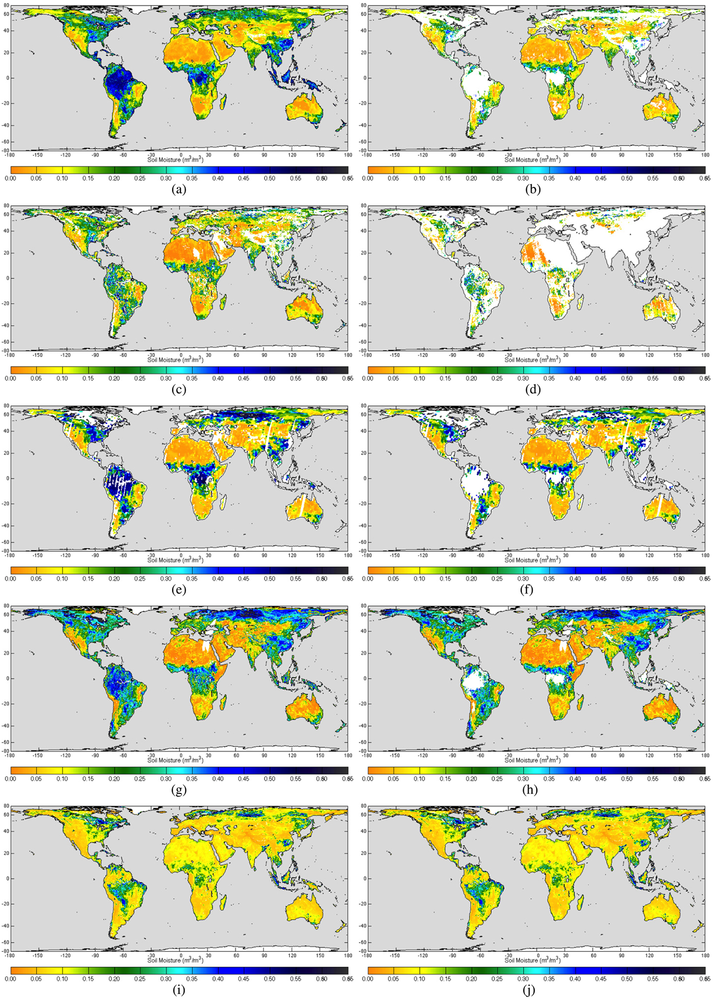
Global patterns of soil moisture retrieved by (a) and (b) SMAP, (c) and (d) SMOS, (e) and (f) Aquarius, (g) and (h) ASCAT, and (i) and (j) AMSR2 over a 1-week period from June 1 to 7, 2015. (a), (c), (e), (g), and (i) Nominal and (b), (d), (f), (h), and (j) masked soil moisture maps are shown. ASCAT-derived soil moisture data in (g) and (h) are converted from soil moisture index (see the text). The AMSR2 masked data are identical to the nominal data since AMSR2 is provided without flags.
A. Soil Moisture Active Passive
SMAP observes the Earth at L-band frequency, its nominal incidence angle is 40°, and global coverage is achieved on average every 2–3 days. The soil moisture product investigated here is the validated release of the L2 passive soil moisture product (L2_SM_P) posted on a 36-km Earth-fixed grid using the global cylindrical Equal-Area Scalable Earth Grid projection Version 2 (EASEv2) [8]. SMAP is on a Sun-synchronous orbit with 6:00 A.M. (descending)/6:00 P.M. (ascending) local equatorial overpass times; vertical profiles of soil temperature and dielectric properties are expected to be more uniform during early morning overpasses than during other times of the day [9]. The SMAP soil moisture retrieval algorithms are based on the simplified radiative transfer equation known as the τ-ω model. Of the five soil moisture retrieval algorithms produced for the SMAP L2_SM_P product, only the baseline V-pol single-channel algorithm (SCA-V) is discussed because the most recent assessment based on in situ data from core validation sites indicated that it is the best overall option [10]. SMAP data version 3.0 (composite release ID: 13080) was used for this analysis; it is available through the NASA Distributed Active Archive Center (DAAC) at the National Snow and Ice Data Center (NSIDC) [11]. The “recommended for retrieval” quality flag provided with the product was used in this study to consider only those pixels that are expected to meet the performance requirement of the mission. Pixels with static water fraction <5%, coastal proximity >36 km, urban fraction <50%, precipitation/snow/permanent ice/frozen ground fraction <5%, slope standard deviation <3°, vegetation water content (VWC) <5 kg/m2, and converged geophysical inversion are considered “recommended for retrieval.” A detailed description of the flags used in the L2_SM_P product can be found in [10]–[12]. For this comparison, the 6:00 A.M. overpass is considered and the orbit closest to 6:00 A.M. is chosen when selecting the other satellite soil moisture products. Example nominal and masked SMAP data for June 1–7, 2015 are shown in Fig. 1(a) and (b). Nominal data indicate unflagged data and masked data denote data after application of the product-specific QC mask.
B. Soil Moisture and Ocean Salinity
The SMOS spacecraft was launched on November 2, 2009 by ESA, CNES, and CTDI to primarily map soil moisture and ocean salinity, but also many other secondary geophysical parameters [13], [14]. SMOS observes the Earth with a synthetic aperture in the 1.4-GHz (L-band) range and with multiple incidence angles ranging from 0° to 65°. SMOS measures all stokes vectors of the brightness temperature on a Sun-synchronous orbit with 6:00 A.M. (ascending)/6:00 P.M. (descending) local equatorial times and achieves global coverage every 3 days. The SMOS soil moisture retrieval algorithm is based on the τ-ω model. In essence, the algorithm utilizes an iterative approach where the sum of squared weighted differences between measured and modeled brightness temperature data is minimized for a variety of incidence angles [15]. The reader is referred to the SMOS L2 processor soil moisture ATBD [16] for more details on the SMOS soil moisture retrieval algorithm. Data version v300 of the SMOS L3 soil moisture product posted on a 25-km Earth-fixed EASEv2 grid (P11p) available from the Centre Aval de Traitement des Données SMOS [17] was used. In this study, the product was regridded to EASEv2 at 36 km by bilinear interpolation and a conservative flagging was applied. Pixels were included only if: 1) VWC <5 kg/m2 or classified as vegetated surfaces or temperate forests in the ECOCLIMAP land use map [18], [19] (S_Tree_1= =11 or S_Tree_1= =12); 2) under nominal conditions, hence discarding pixels that are barren, snow covered, or frozen, or that contain dense forest, high topography, or too much open water (Science_Flags (Bit 1)= =0); and 3) with an RFI probability <10% (Rfi_Prob<0.1). Example nominal and masked SMOS data for June 1–7, 2015 are shown in Fig. 1(c) and (d).
C. Aquarius/Satélite de Aplicaciones Científicas-D
NASA’s Aquarius instrument on board the Argentine SAC-D satellite was launched on June 10, 2011. It carried an L-band radar and an L-band radiometer and observed the Earth with three beams at different resolutions and incidence angles (29.36°, 38.49°, and 46.29°). Together, they formed a 390-km ground swath with an exact 7-day repeat orbit. Aquarius primarily aimed at providing global measurements of sea surface salinity [20], but it also produced a global soil moisture product based on the radiometer observations [21]. Aquarius was on a Sun-synchronous orbit with 6:00 A.M. (descending)/6:00 P.M. (ascending) local overpass times. The Aquarius soil moisture retrieval algorithm is based on the τ–ω model and is implemented as an H-pol single-channel algorithm (SCA-H). For more details, the reader is referred to the Aquarius VSM ATBD [22]. For this study, the Aquarius L2 soil moisture product, available through the NASA DAAC at the NSIDC [23], was regridded to EASEv2 at 36 km by averaging the data using inverse distance weighting for each day. Flags from the Aquarius soil moisture and radiometer products were applied during regridding: only pixels with VWC <5 kg/m2 (Radiometer_flags Bit 0), land fraction >90%, and containing no RFI were considered. The Aquarius satellite ceased operation on June 7, 2015, and hence it overlaps with the SMAP data set for a little more than two months, from April 1, 2015 to June 7, 2015. Example nominal and masked Aquarius data for June 1–7, 2015 are shown in Fig. 1(e) and (f).
D. European Meteorological Operational (MetOp-B) Advanced Scatterometer
ESA’s and EUMETSAT’s European Meteorological Operational-B spacecraft carrying the ASCAT was launched on September 17, 2012. ASCAT is a real aperture radar, operating at 5.3 GHz (C-band) using vertically polarized antennas. It set out to measure wind speed and wind direction over the oceans, but also provides a global soil moisture index. It observes the Earth on a Sun-synchronous orbit with 9:30 A.M. (descending)/9:30 P.M. (ascending) local overpass times and has a temporal revisit of 3 days. The ASCAT soil moisture retrieval algorithm is based on a physically motivated change detection algorithm for use with C-band scatterometers developed by Vienna University of Technology (TU Wien). More information on the soil moisture retrieval algorithm can be found in the ATBD [24]. The ASCAT L2 soil moisture index, available through the EUMETSAT Earth Observation portal [25], was regridded to EASEv2 at 36 km by interpolating the data using inverse distance weighting for each day. Additionally, pixels were masked if the probability of snow, frozen ground, wetland, and increased topography >50%, and if the soil moisture estimation uncertainty due to other sources >50%. Soil porosity on EASEv2 grid at a 9-km resolution is delivered as ancillary data to the SMAP L4 soil moisture product [26], [27]; it was averaged to 36 km and multiplied with the soil moisture index. Hence, the ASCAT soil moisture index on EASEv2 grid at 36 km was converted into volumetric soil moisture by multiplication with soil porosity. Note that this soil moisture product is not the official ASCAT product and will have embedded within it errors originating from the soil porosity product. Other satellite soil moisture products considered in this study may also contain errors originating from their respective soil texture ancillary data sets and dielectric models. Example nominal and masked ASCAT-derived data for June 1–7, 2015 are shown in Fig. 1(g) and (h).
E. Advanced Microwave Scanning Radiometer 2
The AMSR2 instrument was launched on JAXA’s Global Change Observation Mission-Water Shizuku (GCOM-W1) spacecraft on May 18, 2012. AMSR2 is similar to the JAXA-provided AMSR2-EOS (AMSR-E) instrument launched in 2002 on the NASA EOS Aqua satellite [28]. AMSR2 has 7 frequencies and 14 channels, and 1:30 A.M. (descending)/1:30 P.M. (ascending) local overpass times at the equator. The incidence angle is fixed at 55° and global coverage is achieved every 2–3 days. The AMSR2 soil moisture retrieval algorithm utilizes the 10.65- (H- and V-pol) and 36.5-GHz (V-pol) channels and simultaneously retrieves soil moisture and VWC from two indices that are derived from polarization and frequency brightness temperature differences. More information on the soil moisture retrieval algorithm can be found in the description of the GCOM-W1 AMSR2 Level 1R and L2 algorithms [29]. In this study, the AMSR2 L3 soil moisture posted at 0.25°, available through the GCOM-W1 Data Providing Service [30], was regridded to EASEv2 at 36 km by bilinear interpolation. No flags are provided in the AMSR2 soil moisture. The AMSR2 soil moisture product is reported to have some known issues (i.e., overestimation over deserts) [31], [32]. It should be noted that such algorithm incompleteness can have a larger impact on soil moisture comparisons than differences between satellites, such as frequency or retrieval type. Example nominal and masked AMSR2 data for June 1–7, 2015 are shown in Fig. 1(i) and (j). In this case, since no flags are provided, the masked data are identical to the nominal data.
III. Soil Moisture Intercomparison
This section describes comparison results between SMAP L2_SM_P and other satellite-based soil moisture products.
A. Global Patterns and Statistics
Global maps of soil moisture serve as a first qualitative step in assessment. Fig. 1 shows global composites of the nominal and masked soil moisture over a 1-week period from June 1–7, 2015; it will be discussed in detail in the following paragraphs. Global coverage is achieved by SMAP in 2–3 days; however, a 1-week period was chosen so that the same coverage of soil moisture by SMAP and all other satellites can be compared; Aquarius requires 1 week for global coverage. Figs. 1(a), (c), (e), (g), and (i) show nominal pixels, while Figs. 1(b), (d), (f), (h), and (j) show pixels after the application of the product-specific QC flags; the white areas indicate where data has been masked. The nominal retrievals have to be interpreted with caution as they contain pixels with surface/instrument conditions (e.g., mountainous terrain, dense vegetation, RFI, and frozen ground) that can lead to inaccurate soil moisture retrievals. The root-mean-square difference (RMSD), unbiased RMSD (ubRMSD), bias, and correlation (R) between SMAP and the other satellite products after the application of product-specific QC flags are shown in Figs. 2 and 3, respectively, which were taken from April 1, 2015 to April 1, 2016 for SMAP with SMOS, ASCAT, and AMSR2 and from April 1, 2015 to June 7, 2015 for SMAP and Aquarius. Results in Figs. 2 and 3 include only pixels where both data sets have valid retrievals after masking. Other more advanced metrics, such as triple collocation, generally require a longer record period and were therefore not utilized in this study focusing on the first year of operation. It is furthermore emphasized that the comparison periods of Figs. 1–3 are very different: Fig. 1 compares global patterns over a 1-week period, while Figs. 2 and 3 present statistics over a longer time span (1 year for SMAP with SMOS, ASCAT, and AMSR2, and a little more than 2 months for SMAP with Aquarius). This should be considered in the following analysis.
Fig. 2.
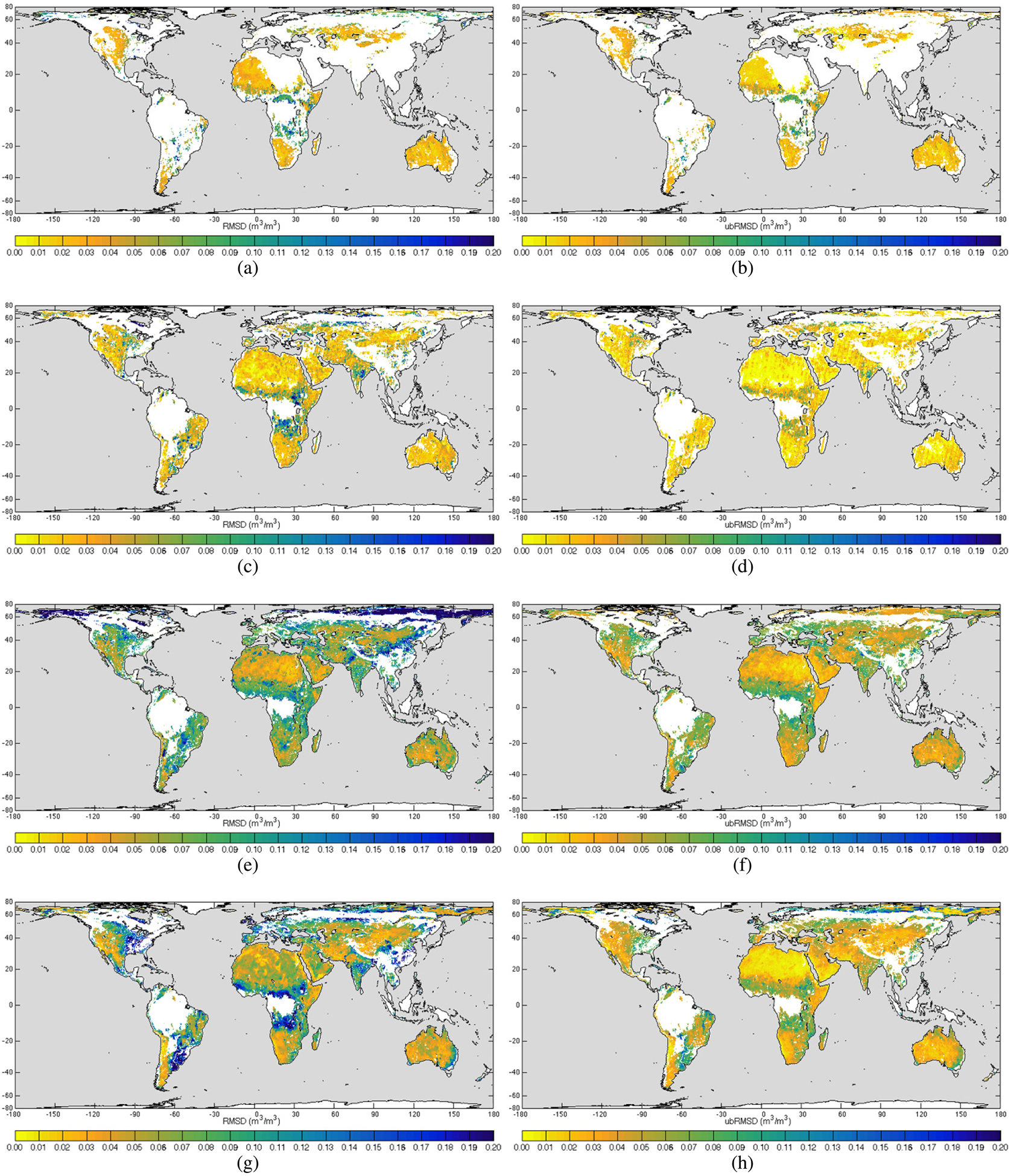
Global statistics of RMSD and ubRMSD for SMAP with SMOS, Aquarius, ASCAT and AMSR2. Statistics are calculated for April 1, 2015–April 1, 2016 for SMAP with SMOS, ASCAT, and AMSR2, and for April 1–June 7, 2015 for SMAP with Aquarius. (a) RMSD of SMAP and SMOS. (b) ubRMSD of SMAP and SMOS. (c) RMSD of SMAP and Aquarius. (d) ubRMSD of SMAP and Aquarius. (e) RMSD of SMAP and ASCAT. (f) ubRMSD of SMAP and ASCAT. (g) RMSD of SMAP and AMSR2. (h) ubRMSD of SMAP and AMSR2.
Fig. 3.
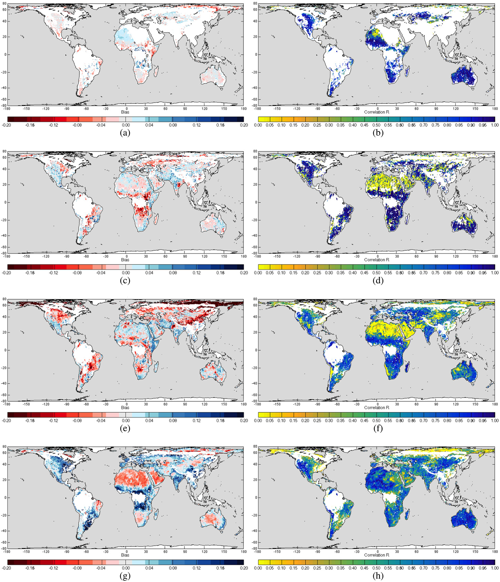
Global statistics of bias and correlation (R) for SMAP with SMOS, Aquarius, ASCAT, and AMSR2. Statistics are calculated for April 1, 2015–April 1, 2016 for SMAP with SMOS, ASCAT, and AMSR2, and for April 1–June 7, 2015 for SMAP with Aquarius. Bias is defined as the difference between SMAP and the compared soil moisture product; red indicates SMAP with lower soil moisture and blue indicates SMAP with higher soil moisture. (a) Bias of SMAP and SMOS. (b) Correlation R of SMAP and SMOS. (c) Bias of SMAP and Aquarius. (d) Correlation R of SMAP and Aquarius. (e) Bias of SMAP and ASCAT. (f) Correlation R of SMAP and ASCAT. (g) Bias of SMAP and AMSR2. (h) Correlation R of SMAP and AMSR2.
The nominal soil moistures of SMAP and SMOS [Fig. 1(a) and (c)] compare well over most land cover types, but differences are apparent over the northern latitudes (Alaska, Russian Taiga, and Tundra), for densely vegetated areas (Amazon, Congo, and Indonesia), and areas where SMOS is impacted by RFI (such as parts of Europe, the Middle East, and Asia). Similar observations were made by Leroux et al. [33]. Both the SMAP and SMOS soil moisture retrieval algorithms are based on the τ-ω model, but they employ different land cover maps to select their respective (τ, ω, and h) parameters; SMAP uses the International Geosphere Biosphere Program (IGBP) classification [3], [34] and SMOS uses ECOCLIMAP. This can in part explain some of the observed differences, especially over the northern latitudes and densely vegetated areas. The masked soil moistures of SMAP and SMOS [Fig. 1(b) and (d)] show differences in coverage: SMOS shows masked areas over Northeast Africa, Europe, Middle East, and Asia, whereas much of the dense forest in the Amazon and central Africa is not masked. These differences in coverage are due to differences in the product-specific QC flags. The RMSD, ubRMSD, and R in Figs. 2(a) and (b) and 3(b) suggest similar conclusions. SMOS generally shows a slightly wetter trend than SMAP, with the exception of a drier trend for desert-like biomes and denser vegetated regions, as seen in Fig. 3(a).
Aquarius [Fig. 1(e) and (f)] compares well with SMAP [Fig. 1(a) and (b)] for bare to moderately vegetated areas, but shows higher soil moisture over denser vegetation. This can also be observed from the RMSD, ubRMSD, and bias maps in Figs. 2(c) and (d) and 3(c). Note that the bias in Figs. 2(c) and (d) and 3(c) is calculated for a little over two months and should only be used to investigate general trends. Similar to SMAP, Aquarius operates at L-band with an algorithm based on the τ-ω model, but uses different (τ, ω, h) parameters due to its coarser resolution. Differences in algorithm parameter could explain differences in soil moisture patterns that are tied to land cover type. The R in Fig. 3(d) is generally very high, but is low over the Sahara since desert-like biomes exhibit a very small dynamic range.
SMAP [Fig. 1(a) and (b)] and ASCAT [Fig. 1(g) and (h)] show similar spatial patterns, but ASCAT tends to be wetter (and drier) than SMAP. Specifically, ASCAT is wetter in the high northern latitudes and over moderate to dense vegetation and drier over desert-like regions, i.e., it exhibits a greater dynamic range at both wet and dry ends. This can also be observed from the RMSD, ubRMSD, and bias maps in Figs. 2(e) and (f) and 3(e). ASCAT operates at a higher frequency (C-band) at which electromagnetic waves are not expected to be able to penetrate far into or originate from deep inside denser vegetation. SMAP at L-band is capable of retrieving soil moisture within the accuracy requirement for areas with VWC up to 5 kg/m2. The R between SMAP and ASCAT in Fig. 3(f) is low over bare soil regions; as mentioned in the previous paragraph, this is due to desert-like biomes exhibiting a very small dynamic range. In addition, scatterometer signals such as from ASCAT can become more sensitive to scattering from deeper soil layers under extremely dry conditions; this can further decrease correlation [35].
AMSR2 [Fig. 1(i) and (j)] shows a compressed soil moisture range compared with SMAP [Fig. 1(a) and (b)] and the other satellite products. It exhibits an overall dry bias, but over desert areas it is wetter than SMAP, as shown in Fig. 3(g). The RMSD and ubRMSD in Figs. 2(g) and (h) show low to moderate RMSDs over desert areas and larger differences with increasing vegetation. The R in Fig. 3(h) is highest in dry areas, low in the northern latitudes, and moderate over the rest of the Earth. The AMSR2 product does not contain any flags to further assess the quality of the product.
For all subsequent analyses, the product-specific QC-masked data sets are used.
B. Transect Comparison
Transect comparisons, while localized in space, can indicate the relative performance of soil moisture retrieval algorithms over different biomes. For this purpose, a transect through the African continent spanning from the Saharan desert and semiarid Sahel in the north, through the Sudanian Savanna, Congolian rainforest, and the flood deltas of the Zambezi and Okavango rivers to the Namibian desert in the south, was selected. Plots of soil moisture versus latitude for SMAP, SMOS, Aquarius, ASCAT, and AMSR2 for May 5–11, 2015 after the application of product-specific QC flags are shown in Fig. 4. This transect is especially interesting as it cuts across the Zambezi and Okavango floodplains that are influenced by the monsoon season of southeast Asia (late October to April) [36]. During this time, floods are frequent and surface water covers most of the flood plain. In May, the dry season is generally underway and surface water is disappearing, but high soil moisture is still expected; this can be clearly seen in Fig. 4. Toward July/August, the floodplains are generally dry and the average soil moisture should be at its minimum in late August/September. Fig. 5 shows the SMAP soil moisture after the application of SMAP-specific QC flags for April 1, 2015–April 1, 2016; the expected dry and wet seasons of the Zambezi and Okavango floodplains can be clearly observed.
Fig. 4.
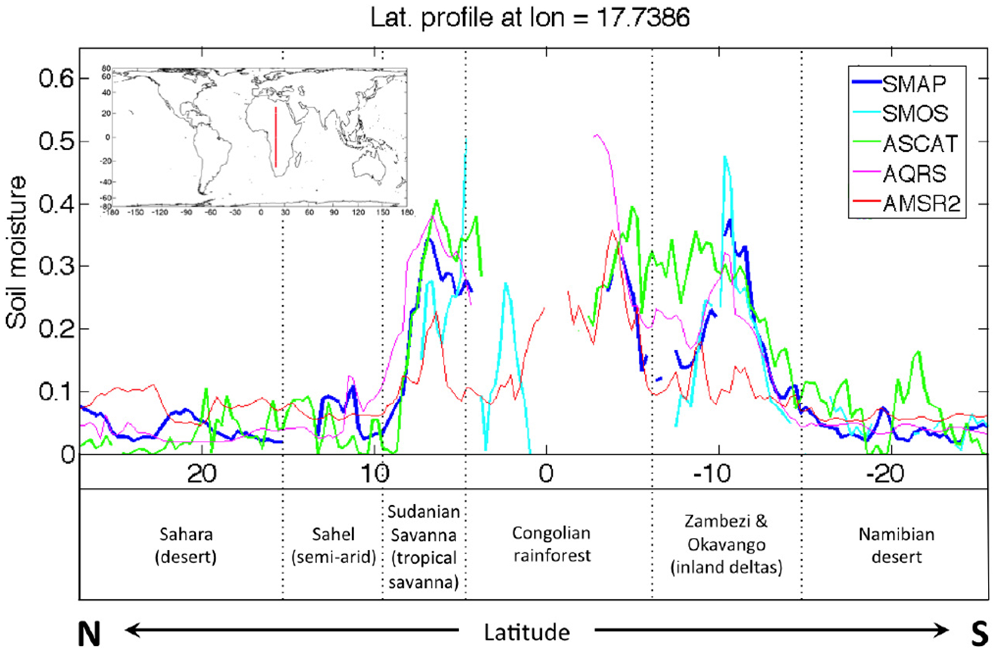
(Top) North–south transect across Africa at lon = 17.7386° (red line in top left inset) showing SMAP, SMOS, Aquarius (AQRS), ASCAT, and AMSR2 soil moisture after the application of product-specific QC flags for May 5–11, 2015. (Bottom) Approximate location of major biomes.
Fig. 5.
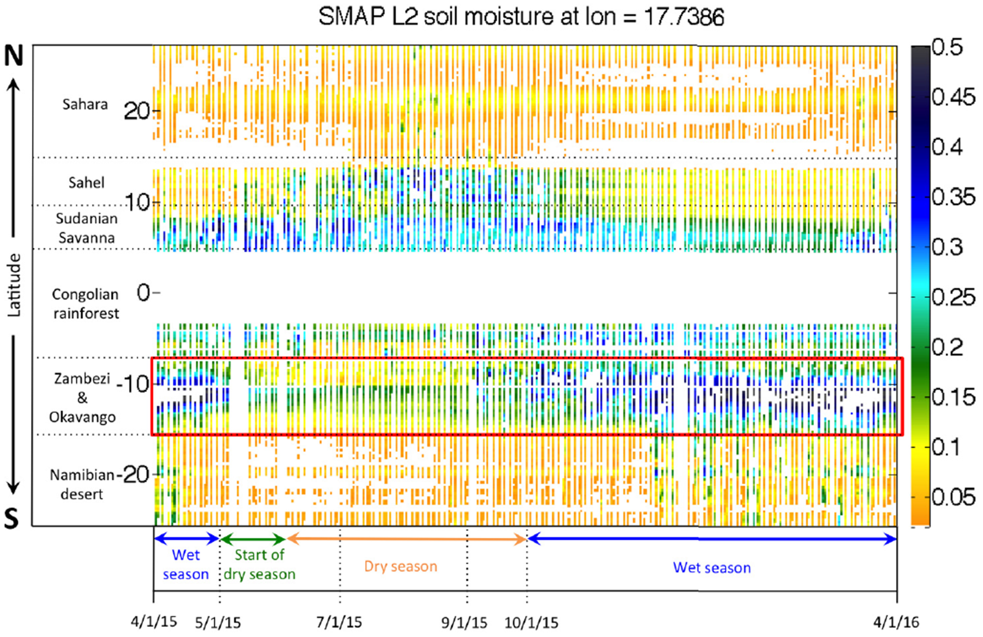
(Top) North–south transect across Africa at lon = 17.7386° showing SMAP soil moisture after the application of SMAP-specific QC flags for April 1, 2015-April 1, 2016. The white areas represent masked pixels. (Left) Approximate latitude bands of the major biomes. The red box outlines the location of the Zambezi and Okavango floodplains. (Bottom) Expected dry and wet seasons of the Zambezi and Okavango floodplains.
SMAP and SMOS show similar sharp soil moisture transitions when crossing into/out-of denser vegetated areas. SMOS exhibits a few very dry pixels over the Congolian rainforest where most other satellite products are masked. On the other hand, many SMOS pixels over the Sahara and Sahel are masked due to RFI. For the remaining pixels, SMAP and SMOS compare well, with SMOS exhibiting wetter soil moisture over the floodplains and at the northern onset of the Congolian rainforest.
SMAP and Aquarius show similar transitions, although some differences can be observed in the Sudanian Savanna and the floodplains. Aquarius tends to be overall wetter than SMAP. This is especially visible in the region between the Congolian rainforest and the floodplains where Aquarius does not decrease to the lower soil moisture level of SMAP and SMOS.
SMAP and ASCAT show similar overall trends, but ASCAT exhibits a more variable soil moisture signal. This can be seen in the Sahara where the ASCAT soil moisture seems to fluctuate more than the soil moisture by SMAP. ASCAT is much wetter than SMAP, SMOS, and Aquarius in the region between the Congolian rainforest and the floodplains; its soil moisture does not decrease as the other soil moisture products indicate. ASCAT furthermore shows a soil moisture peak of 0.16 cm3/cm3 in the Namibian desert, which is not seen in any other soil moisture product.
SMAP and AMSR2 largely disagree in their soil moisture spatial patterns. AMSR2 exhibits a persistent wet bias for the drier regions such as the Sahara, Sahel, and the Namibian desert and a consistent dry bias for the denser vegetated biomes. Furthermore, it does not show any sensitivity over the floodplain deltas.
C. Intercomparison of SMAP With Existing Satellite-Based Soil Moisture Products by IGBP Land Cover Type
Statistics such as ubRMSD, bias, RMSD, and R are calculated over 1 year, specifically April 1, 2015–April 1, 2016, for SMAP with SMOS, ASCAT, and AMSR2. SMAP and Aquarius only overlap for a little more than two months (April 1, 2015–June 7, 2015), and hence the statistics are derived for that time period. The statistics are calculated by IGBP classification, as given in Table II, and are listed in Table III. It is noted that the number of data point pairs can vary depending on land cover class and the applied product-specific QC flags.
TABLE II.
IGBP Classification
| Acronym | IGBP land cover class |
|---|---|
| ENF | Evergreen Needleleaf Forest |
| EBF | Evergreen Broadleaf Forest |
| DNF | Deciduous Needleleaf Forest |
| DBF | Deciduous Broadleaf Forest |
| MXF | Mixed Forest |
| CSH | Closed Shrublands |
| OSH | Open Shrublands |
| WSV | Woody Savannas |
| SAV | Savannas |
| GRS | Grasslands |
| PEW | Permanent Wetlands |
| CRP | Croplands |
| URB | Urban and Built-up |
| MOS | Cropland / Natural Vegetation Mosaic |
| SNI | Snow and Ice |
| BAR | Barren or Sparsely Vegetated |
TABLE III.
Intercomparison of SMAP With SMOS, Aquarius, ASCAT, and AMSR2 by IGBP Land Cover Type. Comparison of SMAP With SMOS, ASCAT, and AMSR2 for April 1, 2015–April 1, 2016 and SMAP and Aquarius for April 1, 2015–June 7, 2015. Land Cover Classes to Be Treated Carefully Are Shaded in Gray
| IGBP LandCover | obRMSD (m3/m3) | bias (m3/m3) | RMSD (m3/m3) | R | Number of data point pairs | |||||||||||||||
|---|---|---|---|---|---|---|---|---|---|---|---|---|---|---|---|---|---|---|---|---|
| Class | SMOS | Aquarius | ASCAT | AMSR2 | SMOS | Aquarius | ASCAT | AMSR2 | SMOS | Aquarius | ASCAT | AMSR2 | SMOS | Aquarius | ASCAT | AMSR2 | SMOS | Aquarius | ASCAT | AMSR2 |
| NaN | 0.093 | NaN | 0.078 | 0.840 | 0626 | 0 | 572 | |||||||||||||
| NaN | 0.099 | NaN | 0.107 | NaN | 0.265 | 0 | 62 | |||||||||||||
| 0.066 | 0.117 | 0.023 | 0.086 | 0.926 | 0.548 | 99 | 444 | |||||||||||||
| CSH | 0.088 | 0.034 | 0.064 | 0.046 | −0.042 | 0.029 | 0.066 | 0.060 | 0.097 | 0.045 | 0.092 | 0.075 | 0.673 | 0.917 | 0.418 | 0.480 | 457 | 147 | 2282 | 3369 |
| OSH | 0.0S2 | 0.043 | 0.135 | 0.069 | −0.029 | 0.007 | −0.065 | 0.003 | 0.060 | 0.044 | 0.150 | 0.069 | 0.831 | 0.815 | 0.582 | 0.463 | 191909 | 38615 | 777197 | 1173315 |
| WSV | 0.097 | 0.090 | 0.132 | 0.119 | 0.040 | −0.038 | −0.034 | 0.081 | 0.105 | 0.098 | 0.136 | 0.144 | 0.754 | 0.793 | 0.501 | 0.222 | 66666 | 17077 | 300499 | 446432 |
| SAY | 0.071 | 0.068 | 0.085 | 0.084 | −0.004 | −0.023 | −0.026 | 0.028 | 0.071 | 0.072 | 0.089 | 0.088 | 0.799 | 0.815 | 0.745 | 0.513 | 47191 | 21743 | 344310 | 522317 |
| GRS | 0.050 | 0.051 | 0.087 | 0.072 | −0.008 | 0.010 | −0.028 | 0.041 | 0.050 | 0.051 | 0.092 | 0.083 | 0.880 | 0.827 | 0.676 | 0.489 | 90949 | 32259 | 542195 | 900959 |
| CRP | 0.055 | 0.077 | 0.099 | 0.081 | 0.005 | −0.015 | −0.030 | 0.085 | 0.055 | 0.078 | 0.103 | 0.117 | 0.818 | 0.786 | 0.588 | 0.486 | 44281 | 28987 | 430160 | 733367 |
| MOS | 0.076 | 0.092 | 0.101 | 0.098 | −0.003 | −0.004 | −0.021 | 0.090 | 0.076 | 0.092 | 0.103 | 0.133 | 0.794 | 0.763 | 0.678 | 0.449 | 18784 | 9410 | 157002 | 257879 |
| BAR | 0.024 | 0.028 | 0.059 | 0.042 | 0.019 | 0.004 | 0.011 | −0.028 | 0.030 | 0.028 | 0.060 | 0.050 | 0.808 | 0.497 | 0.313 | 0.436 | 65269 | 47488 | 716970 | 1147453 |
| All | 0.066 | 0.064 | 0.108 | 0.087 | −0.005 | −0.006 | −0.030 | 0.028 | 0.067 | 0.065 | 0.112 | 0.091 | 0.802 | 0.838 | 0.649 | 0.407 | 528300 | 196740 | 3287364 | 5217208 |
Generally, the forested classes (ENF, EBF, DNF, DBF, and MXF) contain fewer pixels than other classes due to masking schemes of the satellite products. The statistics in the forested classes have to therefore be treated with caution. The permanent wetland (PEW) class performs overall poorly, accumulating very high ubRMSDs, biases, and RMSDs, and low or negative Rs across all comparisons. PEWs usually contain standing water or marsh conditions over which soil moisture retrieval algorithms may perform poorly. The urban and built-up (URB) and snow and ice (SNI) classes are generally masked out in soil moisture products. Pixels where the respective soil moisture algorithm identifies open water surfaces are masked out. Overall, we observe that SMAP compares well with SMOS and Aquarius showing similar values for ubRMSD, bias, and RMSD. SMAP and SMOS show lower ubRMSDs and higher R for barren or sparsely vegetated soils (BAR), cropland/natural vegetation mosaic (MOS), and cropland and grassland (CRP, GRS), while SMAP and Aquarius agree better for savannas (SAV), woody SAV (WSV), and the shrubland classes (OSH, CSH). The R of SMAP and Aquarius seems to be slightly higher than SMAP and SMOS, although this is likely due to SMAP and Aquarius only overlapping for two months and significant differences in satellite resolutions.
SMAP agrees less with ASCAT and AMSR2. SMAP and AMSR2 show lower ubRMSD values across all IGBP classes than SMAP with ASCAT, likely due a slight improvement when removing the bias between SMAP and AMSR2. SMAP and ASCAT show higher R values than SMAP and AMSR2 for most land cover classes.
D. Seasonal Intercomparison of SMAP With Existing Satellite-Based Soil Moisture Products
A seasonal analysis of the comparison statistics for SMAP with SMOS, ASCAT, and AMSR2 over the available 1-year period is conducted; April 1, 2015–April 1, 2016. In this analysis, the northern and southern hemispheres are separated to avoid mixing seasonal variations of the hemispheres. Furthermore, the forested classes (ENF, EBF, DNF, DBF, and MXF), the PEW class, the URB class, the SNI class, and pixels where the respective soil moisture algorithm identifies open water surfaces are excluded when calculating the statistics shown in Tables IV and V.
TABLE IV.
Seasonal Intercomparison of SMAP With SMOS, ASCAT, and AMSR2 for April 1, 2015–April 1, 2016. Only the Northern Hemisphere Is Considered and the IGBP Classes ENF, EBF, DNF, DBF, MXD, PEW, URB, AND SNI, and Pixels Where the Respective Soil Moisture Algorithm Identifies Open Water Surfaces Are Excluded
| Metrics | Mar-Apr-May | Jun-Jul-Aug | Sep-Oct-Nov | Dec-Jan-Feb | All | ||||||||||
|---|---|---|---|---|---|---|---|---|---|---|---|---|---|---|---|
| SMOS | ASCAT | AMSR2 | SMOS | ASCAT | AMSR2 | SMOS | ASCAT | AMSR2 | SMOS | ASCAT | AMSR2 | SMOS | ASCAT | AMSR2 | |
| ubRMSD (m3/m3) | 0.060 | 0.092 | 0.084 | 0.070 | 0.132 | 0.094 | 0.063 | 0.098 | 0.078 | 0.055 | 0.073 | 0.087 | 0.065 | 0.114 | 0.087 |
| Bias (m3/m3) | −0.001 | −0.006 | 0.035 | −0.021 | −0.082 | 0.012 | −0.005 | −0.033 | 0.033 | 0.004 | 0.019 | 0.038 | −0.009 | −0.037 | 0.027 |
| RMSD (m3/m3) | 0.060 | 0.092 | 0.091 | 0.073 | 0.156 | 0.095 | 0.063 | 0.103 | 0.084 | 0.055 | 0.075 | 0.095 | 0.065 | 0.119 | 0.091 |
| Correlation R | 0.845 | 0.697 | 0.404 | 0.725 | 0.574 | 0.387 | 0.810 | 0.700 | 0.468 | 0.822 | 0.721 | 0.281 | 0.789 | 0.630 | 0.379 |
TABLE V.
Seasonal Intercomparison of SMAP With SMOS, ASCAT, and AMSR2 for April 1, 2015–April 1, 2016. Only the Southern Hemisphere Is Considered and the IGBP Classes ENF, EBF, DNF, DBF, MXD, PEW, URB, and SNI, and Pixels Where the Respective Soil Moisture Algorithm Identifies Open Water Surfaces Are Excluded
| Metrics | Mar-Apr-May | Jun-Jul-Aug | Sep-Oct-Nov | Dec-Jan-Feb | All | ||||||||||
|---|---|---|---|---|---|---|---|---|---|---|---|---|---|---|---|
| SMOS | ASCAT | AMSR2 | SMOS | ASCAT | AMSR2 | SMOS | ASCAT | AMSR2 | SMOS | ASCAT | AMSR2 | SMOS | ASCAT | AMSR2 | |
| ubRMSD (m3/m3) | 0.067 | 0.085 | 0.086 | 0.060 | 0.074 | 0.077 | 0.057 | 0.071 | 0.078 | 0.069 | 0.080 | 0.092 | 0.064 | 0.079 | 0.083 |
| Bias (m3/m3) | −0.006 | −0.027 | 0.023 | 0.003 | 0.008 | 0.034 | 0.013 | 0.008 | 0.036 | −0.003 | −0.018 | 0.036 | 0.002 | −0.007 | 0.032 |
| RMSD (m3/m3) | 0.067 | 0.089 | 0.089 | 0.060 | 0.074 | 0.084 | 0.059 | 0.071 | 0.085 | 0.069 | 0.082 | 0.099 | 0.064 | 0.079 | 0.089 |
| Correlation R | 0.823 | 0.749 | 0.483 | 0.790 | 0.700 | 0.420 | 0.814 | 0.730 | 0.532 | 0.845 | 0.786 | 0.502 | 0.825 | 0.747 | 0.489 |
The comparison of SMAP and SMOS, and SMAP and ASCAT shows a seasonal variation; they agree better during the spring and winter months in both hemispheres (December–May in the northern hemisphere and June–November in the southern hemisphere), as observed by lower ubRMSD, RMSD, bias, and higher R during these months. This points toward retrieval differences over vegetated classes that show an increased/decreased biomass during the summer and autumn months. Albergel et al. [37] assessed seasonal variability of SMOS and ASCAT with in situ soil moisture in 2010 and observed a similar trend. It is interesting to note that the lowest ubRMSD and RMSD and the highest R coincide in the same months (December–May) on the northern hemisphere. In contrast, on the southern hemisphere, the lowest ubRMSD and RMSD fall into June to November, while the highest R falls into December to May. The comparison of SMAP and AMSR2 shows some seasonal variation, but it is not clear which contributing factors lead to this behavior. Excluding several IGBP classes when calculating these statistics, we observe that SMAP and SMOS compare better than SMAP and ASCAT or SMAP and AMSR2. This does not point toward a superiority of any particular product; it assesses the SMAP L2_SM_P product in context with the other satellite soil moisture products globally over diverse biomes.
IV. Conclusion
This paper provides the first intercomparison between the passive SMAP soil moisture product and soil moisture products from SMOS, Aquarius, ASCAT, and AMSR2. Detailed analyses spanning investigations of global patterns and statistics, transect comparisons and assessments of land cover dependence, and seasonal variations reveal differences and similarities between the intercompared soil moisture products.
In summary, SMAP and SMOS appear to be the most similar among the five soil moisture products considered in this paper, exhibiting the smallest ubRMSD and highest R overall. Observed differences such as low/high soil moisture over densely vegetated areas such as the Amazon and the Congolian forests can in part be explained by the use of different land cover type maps in the respective soil moisture retrieval algorithms. Overall, SMOS tends to be slightly wetter than SMAP, excluding forests. A significant difference between SMAP and SMOS is SMAP’s use of sophisticated RFI filtering hardware and software allowing it to acquire brightness temperature observations that are relatively free of RFI.
SMAP and Aquarius overlap only for a little more than two months, and as a result, any conclusions should be made with caution. SMAP and Aquarius compare well especially over low to moderately vegetated areas, but disagree over denser vegetated areas. It is interesting to note that SMAP and SMOS seem to compare better over low vegetated land cover types (such as barren soils, croplands, and grasslands), while SMAP and Aquarius compare more closely over moderately vegetated land cover types (such as savannas and shrublands). However, this conclusion could be in part biased through the overlap of only two summer months between SMAP and Aquarius.
The comparison of SMAP and ASCAT differs from the other comparison pairs, as ASCAT is originally delivered as a soil moisture index, operates at a higher frequency (C-band), and is also the only radar-based soil moisture product within the five intercompared soil moisture products. Ideally and for local comparisons, a porosity from in situ measurements is multiplied with the soil moisture index; the use of a global porosity map is assumed to introduce some errors due to approximations. Despite these withholdings, SMAP and ASCAT show similar overall trends and spatial patterns. ASCAT tends to be wetter than SMAP, especially over moderate to dense vegetation; this may possibly be caused by reduced microwave penetration at C-band. Furthermore, ASCAT exhibits a more variable soil moisture signal.
SMAP and AMSR2 share a similar nominal spatial resolution, but AMSR2 observes at different times of the day and its algorithm operates at higher frequencies (X- and Ka-band); it therefore observes soil moisture from a shallower depth. SMAP and AMSR2 largely disagree in their soil moisture trends and spatial patterns. AMSR2 exhibits an overall dry bias, while desert areas are observed wetter than SMAP. Unfortunately, the AMSR2 product neither applies RFI mitigation nor provides any flags to further assess the quality of the product.
This satellite intercomparison study, in combination with the other four SMAP calibration and validation methodologies, has provided and confirmed insights into the SMAP algorithm. For example, the comparison of the radiometer-only soil moisture to in situ, sparse networks, and soil moisture data from other satellites has resulted in selecting the V-pol SCA-V as the baseline algorithm. These and other analyses have been conducted over the past few years and no further redesigns of the SMAP algorithm based on this study are expected at this point.
Acknowledgment
The authors would like to thank S. Hahn and Dr. W. Wagner at TU Wien for their guidance regarding the ASCAT data set and Dr. T. Maeda and Dr. K. Imaoka from JAXA for their help with the AMSR2 data set. The authors would also like to thank Dr. G. Schumann for providing insights into the monsoon-dependent behavior of the Zambezi and Okavango floodplains.
This work was carried out in part at the Jet Propulsion Laboratory, California Institute of Technology, under a contract with the National Aeronautics and Space Administration.
Biography

Mariko S. Burgin (S’09–M’14) received the M.S. degree in electrical engineering and information technology from the Swiss Federal Institute of Technology (ETH), Zurich, Switzerland, in 2008, and the M.S. and Ph.D. degrees in electrical engineering from the Radiation Laboratory, University of Michigan, Ann Arbor, MI, USA, in 2011 and 2014, respectively.
From 2014 to 2015, she was a Post-Doctoral Scholar with the Water and Carbon Cycles Group, Jet Propulsion Laboratory (JPL), California Institute of Technology, Pasadena, CA, USA. She is currently a Scientist with the Radar Science and Engineering Section at JPL. Her research interests include theoretical and numerical studies of random media, development of forward and inverse scattering algorithms for geophysical parameter retrieval, and the study of electromagnetic wave propagation and scattering properties of vegetated surfaces.

Andreas Colliander (S’04–A’06–M’07–SM’08) received the M.Sc. (Tech.), Lic.Sc. (Tech.), and D.Sc. (Tech.) degrees from the Helsinki University of Technology (TKK; now Aalto University), Espoo, Finland, in 2002, 2005, and 2007, respectively.
He is currently a Research Scientist with the Jet Propulsion Laboratory, California Institute of Technology, Pasadena, CA, USA.
Dr. Colliander is a member of the Science Algorithm Development Team for the Soil Moisture Active Passive (SMAP) mission, focusing on calibration and validation of the geophysical products.

Eni G. Njoku (M’75–SM’83–F’95) received the B.A. degree in natural and electrical sciences from Cambridge University, Cambridge, U.K., in 1972, and the M.S. and Ph.D. degrees in electrical engineering from the Massachusetts Institute of Technology, Cambridge, MA, USA, in 1974 and 1976, respectively.
In 1977, he joined at the Jet Propulsion Laboratory (JPL), California Institute of Technology, Pasadena, CA, USA, where he most recently served as a Senior Research Scientist in the Surface Hydrology Group, before retiring from JPL in 2016. He was a pioneer in soil moisture retrieval algorithm and soil moisture mission development. He was a Project Scientist of the Hydros mission from 2002 to 2006 and the Soil Moisture Active Passive (SMAP) mission from 2008 to 2013. His research interests include passive and active microwave sensing of soil moisture for hydrology and climate applications.
Dr. Njoku was a member of the U.S. Advanced Microwave Scanning Radiometer Science Team. He was a recipient of the NASA Exceptional Public Service Medals in 1985 and 2016.

Steven K. Chan (M’01–SM’03) received the Ph.D. degree in electrical engineering from the University of Washington, Seattle, WA, USA, in 1998, specializing in electromagnetic wave propagation in random media.
He is currently a scientist in hydrology at NASA Jet Propulsion Laboratory, California Institute of Technology, focusing on passive microwave soil moisture retrieval algorithm development. His work in remote sensing of soil moisture encompasses the NASA Aqua/AMSR-E (2002–2011), the JAXA GCOM-W/AMSR2 (2012-present), and more recently the NASA Soil Moisture Active Passive (SMAP) mission (2015-present).

Francois Cabot received the Ph.D. degree in optical sciences from the University of Paris-Sud, Orsay, France, in 1995.
Between 1995 and 2004, he was with the CNES Wide Field of View Instruments Quality Assessment Department, where he was involved in absolute and relative calibration of CNES-operated optical sensors over natural terrestrial targets. In 2004, he joined CESBIO, Toulouse, France, as a SMOS System Performance Engineer through the various stages of the satellite development. He is currently in charge of the design and implementation of the French Center for higher level products for SMOS Data (CATDS). He is also involved in future mission studies to carry out soil moisture measurements with improved resolution and accuracy. His research interests include radiative transfer, both optical and microwave, and remote sensing of terrestrial surfaces.

Yann H. Kerr (M’88–SM’01–F’13) received the engineering degree from École Nationale Supérieur de l’Aéronautique et de l’Espace, Toulouse, France, the M.Sc. degree in electronics and electrical engineering from Glasgow University, Glasgow, Scotland, U.K., and the Ph.D. degree in Astrophysique Géophysique et Techniques Spatiales, Université Paul Sabatier, Toulouse.
From 1980 to 1985, he was with Centre d’Etudes Spatiales de la BIOsphère, Centre National d’Etudes Spatiales (CNES-CESBIO), Toulouse, France. In 1985, he joined Laboratoire d’Etudes et de Recherche en Teledetection Spatiale (LERTS), Toulouse, France, where he was the Director from 1993 to 1994. He spent 19 months at the Jet Propulsion Laboratory, Pasadena, CA, USA, from 1987 to 1988. In 1989, he started to focus on the interferometric concept applied to passive microwave Earth observation and was subsequently the science lead on the MIRAS project for ESA with MMS and OMP. He was also a Co-Investigator on IRIS, OSIRIS, and HYDROS for NASA. He was Science Advisor for MIMR and Co-I on AMSR. Since 1995, he has been with CESBIO, Toulouse, where he was a Deputy Director during 1995–1999 and the Director during 2007–2016. He has been involved with many space missions. His research interests include the theory and techniques for microwave and thermal infrared remote sensing of the Earth, with emphasis on hydrology, water resources management, and vegetation monitoring.
Dr. Kerr is a member of the SMAP Science Team. In 1997, he first proposed the natural outcome of the previous MIRAS work with what was to become the SMOS mission to CNES, a proposal which was selected by ESA in 1999 with him as the SMOS mission Lead-Investigator and the Chair of the Science Advisory Group. He is also in charge of the SMOS science activities coordination in France. He has organized all the SMOS workshops, and was the Guest Editor on three IEEE Special issues and one RSE. He is currently involved in the exploitation of SMOS data and in the Cal/Val activities and related level 2 soil moisture and level 3 and 4 development and SMOS Aquarius SMAP synergistic uses and on the soil moisture essential climate variable. He is also involved in the SMOSNext concept and is involved in both the Aquarius and SMAP missions. He received the GRSS certificate of recognition for leadership in the development of the first synthetic aperture microwave radiometer in space and success of the SMOS mission, and the ESA Team Award. He was nominated the Highly Cited Scientist by Thomson Reuters in 2015.

Rajat Bindlish (SM’05) received the B.S. degree in civil engineering from IIT, Bombay, India, in 1993, and the M.S. and Ph.D. degrees in civil engineering from The Pennsylvania State University, State College, PA, USA, in 1996 and 2000, respectively.
He was with USDA Agricultural Research Service, Hydrology and Remote Sensing Laboratory, Beltsville, MD, USA. He is currently with NASA Goddard Space Flight Center, Greenbelt, MD, USA. His research interests involve the application of microwave remote sensing in hydrology. He is currently working on soil moisture estimation from microwave sensors and their subsequent application in land surface hydrology.

Thomas J. Jackson (SM’96–F’02) received the Ph.D. degree from the University of Maryland, College Park, MD, USA, in 1976.
He is currently a Research Hydrologist with the U.S. Department of Agriculture, Agricultural Research Service, Hydrology and Remote Sensing Laboratory, Beltsville, MD, USA. His research interests include the application and development of remote sensing technology in hydrology and agriculture, and primarily microwave measurement of soil moisture.
Dr. Jackson is a member of the Science and Validation Team of the Aqua, ADEOS-II, Radarsat, Oceansat-1, Envisat, ALOS, SMOS, Aquarius, GCOMW, and SMAP remote sensing satellites. He is a fellow of the Society of Photo-Optical Instrumentation Engineers, the American Meteorological Society, and the American Geophysical Union. In 2003, he was a recipient of the William T. Pecora Award (NASA and Department of Interior) for his outstanding contributions toward understanding the Earth by means of remote sensing, the AGU Hydrologic Sciences Award for his outstanding contributions to the science of hydrology and the IEEE Geoscience and Remote Sensing Society Distinguished Achievement Award in 2011.

Dara Entekhabi (M’04–SM’09–F’15) received the B.S. and M.S. degrees from Clark University, Worcester, MA, USA, and the Ph.D. degree from the Massachusetts Institute of Technology (MIT), Cambridge, MA, USA, in 1990.
He is currently a Professor with the Department of Civil and Environmental Engineering and the Department of Earth, Atmospheric and Planetary Sciences, MIT. He is the Science Team Lead for the National Aeronautics and Space Administration’s Soil Moisture Active Passive mission that was launched in 2015. His research interests include terrestrial remote sensing, data assimilation, and coupled land-atmosphere systems modeling.
Prof. Entekhabi is also a Fellow of the American Meteorological Society and the American Geophysical Union.

Simon H. Yueh (M’92–SM’01–F’09) received the Ph.D. degree in electrical engineering from the Massachusetts Institute of Technology, Cambridge, MA, USA, in 1991.
In 1991, he joined the Massachusetts Institute of Technology, as a Post-Doctoral Research Associate, and joined the Radar Science and Engineering Section at the Jet Propulsion Laboratory, Pasadena, CA, USA. He was the supervisor of Radar System Engineering and Algorithm Development Group from 2002 to 2007, the Deputy Manager of Climate, Oceans and Solid Earth section from 2007 to 2009, and the Section Manager from 2009 to 2013. He was the Project Scientist of the National Aeronautics and Space Administration (NASA) Aquarius mission from 2012 to 2013 and the Deputy Project Scientist of NASA Soil Moisture Active Passive Mission in 2013, and has been the SMAP Project Scientist since 2013. He has been the Principal/Co-Investigator of numerous NASA and DOD research projects on remote sensing of soil moisture, terrestrial snow, ocean salinity, and ocean wind. He has authored four book chapters and published more than 150 publications and presentations.
Dr. Yueh was a recipient of the IEEE GRSS Transaction Prize Paper award in 1995, 2002, 2010, and 2014, the 2000 Best Paper Award in the IEEE International Geoscience and Remote Symposium, the JPL Lew Allen Award in 1998, the Ed Stone Award in 2003, and the NASA Exceptional Technology Achievement Medal in 2014. He is an Associate Editor of IEEE Transactions on Geoscience and Remote Sensing.
Contributor Information
Rajat Bindlish, NASA Goddard Space Flight Center, Greenbelt, MD 20771 USA..
Thomas J. Jackson, U.S. Department of Agriculture, Agricultural Research Service, Hydrology and Remote Sensing Laboratory, Beltsville, MD 20705 USA..
Dara Entekhabi, Massachusetts Institute of Technology, Cambridge, MA 02139 USA..
Simon H. Yueh, NASA Jet Propulsion Laboratory, California Institute of Technology, Pasadena, CA 91109 USA..
References
- [1].Entekhabi D et al. , “The Soil Moisture Active Passive (SMAP) mission,” Proc. IEEE, vol. 98, no. 5, pp. 704–716, May 2010. [Google Scholar]
- [2].Jackson T et al. , “SMAP science data calibration and validation plan,” Jet Propuls. Lab., California Inst. Technol., Pasadena, CA, USA, Tech. Rep. JPL D-52544, 2012. [Google Scholar]
- [3].Entekhabi D, Yueh S, O’Neill P, and Kellogg K, “SMAP handbook,” Jet Propuls. Lab., California Inst. Technol., Pasadena, CA, USA, Tech. Rep 400–1567, 2014. [Google Scholar]
- [4].Colliander A et al. , “Validation of SMAP surface soil moisture products with core validation sites,” Remote Sens. Environ, vol. 191, pp. 215–131, Mar. 2017. [Google Scholar]
- [5].Chen F et al. , “Application of triple collocation in ground-based validation of Soil Moisture Active/Passive (SMAP) level 2 data products,” IEEE J. Sel. Topics Appl. Earth Observ. Remote Sens, vol. 10, no. 2, pp. 489–502, Feb. 2017. [Google Scholar]
- [6].Colliander A et al. , “Validation and scaling of soil moisture in a semiarid environment: SMAP validation experiment 2015 (SMAPVEX15), Remote Sens. Environ, under review. [Google Scholar]
- [7].Pan M, Cai X, Chaney NW, Entekhabi D, and Wood EF, “An initial assessment of SMAP soil moisture retrievals using high-resolution model simulations and in situ observations,” Geophys. Res. Lett, vol. 43, no. 18, pp. 9662–9668, 2016. [Google Scholar]
- [8].Brodzik MJ, Bilingsley B, Haran T, Raup B, and Savoie MH, “EASE-Grid 2.0: Incremental but significant improvements for earth-gridded data sets,” ISPRS Int. J. Geo-Inf, vol. 1, no. 1, pp. 32–45, 2012. [Google Scholar]
- [9].Basharinov AY and Shutko AM, “Simulation studies of the shf radiation characteristics of soils under moist conditions,” NASA Transl. into English of Modelnyye Issledovaniya SVCh Radiatsionnykh Kharacteristik Pochvo-Gruntov v Usloviyakh Uvlazhneniya (Unpublished Report) Moscow, Acad. Sci. USSR, Inst. Radio Eng. Electron., Aug. 1975, pp. 1–81. [Google Scholar]
- [10].Chan SK et al. , “Assessment of the SMAP passive soil moisture product,” IEEE Trans. Geosci. Remote Sens, vol. 54, no. 8, pp. 1–14, Aug. 2016. [DOI] [PMC free article] [PubMed] [Google Scholar]
- [11].O’Neill PE, Chan S, Njoku E, Jackson T, and Bindlish R. NASA, Boulder, CO, USA: SMAP L2 Radiometer Half-Orbit 36 km EASE-Grid Soil Moisture, Version 3, accessed on Jun. 27, 2016 [Online]. Available: 10.5067/PLRS64IU03IT [DOI] [Google Scholar]
- [12].Chan S and Dunbar RS, “SMAP level 2 passive soil moisture product specification document,” Jet Propuls. Lab., California Inst. Technol., Pasadena, CA, USA, Tech. Rep. JPL D-72547, 2015. [Google Scholar]
- [13].Kerr YH et al. , “The SMOS mission: New tool for monitoring key elements ofthe global water cycle,” Proc. IEEE, vol. 98, no. 5, pp. 666–687, May 2010. [Google Scholar]
- [14].Mecklenburg S et al. , “ESA’s Soil Moisture and Ocean Salinity mission: Mission performance and operations,” IEEE Trans. Geosci. Remote Sens, vol. 50, no. 5, pp. 1354–1366, May 2012. [Google Scholar]
- [15].Kerr YH et al. , “The SMOS soil moisture retrieval algorithm,” IEEE Trans. Geosci. Remote Sens, vol. 50, no. 5, pp. 1384–1403, May 2012. [Google Scholar]
- [16].Kerr Y, Waldteufel P, Richaume P, Ferrazzoli P, and Wigneron J-P, SMOS Level 2 Processor Soil Moisture Algorithm Theoretical Basis, Document (ATBD) V4. SM-ESL (CBSA), Toulouse, France, pp. 1–142. [Google Scholar]
- [17].SMOS L3 Product at Centre Aval de Traitement des Données SMOS (CATDS), accessed on Jun. 2016 [Online]. Available: http://www.catds.fr/Products/Available-products-from-CPDC
- [18].Masson V, Champeaux J-L, Chauvin F, Meriguet C, and Lacaze R, “A global database of land surface parameters at 1-km resolution in meteorological and climate models,” J. Climate, vol. 16, no. 9, pp. 1261–1282, 2003. [Google Scholar]
- [19].Faroux S et al. , “ECOCLIMAP-II/Europe: A twofold database of ecosystems and surface parameters at 1 km resolution based on satellite information for use in land surface, meteorological and climate models,” Geosci. Model Develop, vol. 6, no. 2, pp. 563–582, 2013. [Google Scholar]
- [20].Le Vine DM, Lagerloef GSE, Colomb FR, Pellerano FA, and Yueh SH, “Aquarius: An instrument to monitor sea surface salinity from space,” IEEE Trans. Geosci. Remote Sens, vol. 45, no. 7, pp. 2040–2050, Jul. 2007. [Google Scholar]
- [21].Bindlish R, Jackson T, Cosh M, Zhao T, and O’Neill P, “Global soil moisture from the aquarius/SAC-D satellite: Description and initial assessment,” IEEE Geosci. Remote Sens. Lett, vol. 12, no. 5, pp. 923–927, May 2015. [Google Scholar]
- [22].Bindlish R and Jackson TJ, Aquarius VSM Algorithm Theoretical Basis Document Users Guide, Version 2.0, USDA, Beltsville, MD, USA: Hydrol. Remote Sens. Lab, 2013. [Online]. Available: http://nsidc.org/data/docs/daac/aquarius/pdfs/Aquarius_VSM_ATBD_UsersGuide.pdf [Google Scholar]
- [23].Bindlish R and Jackson T. NASA National Snow and Ice Data Center Distributed Active Archive Center Boulder, CO, USA: Aquarius L2 Swath Single Orbit Soil Moisture Data, Version 4, accessed on Jun. 27, 2016 [Online]. Available: 10.5067/Aquarius/AQ2_SM.004 [DOI] [Google Scholar]
- [24].(2013). The EUMETSAT Network on Satellite Application Facilities, Support to Operational Hydrology and Water Management (HSAF), Algorithm Theoretical Basis Document (ATBD) for Product H25/SMOBS-4: METOP ASCAT Soil Moisture Time Series. [Online]. Available: http://hsaf.meteoam.it/documents/ATDD/SAF_HSAF_CDOP_ATBD-25_0_4.pdf
- [25].EUMETSAT Earth Observation Portal (EOP), accessed on Jul. 2016 [Online]. Available: http://www.eumetsat.int/website/home/index.html
- [26].De Lannoy GJM, Koster RD, Reichle RH, Mahanama SPP, and Liu Q, “An updated treatment of soil texture and associated hydraulic properties in a global land modeling system,” J. Adv. Model. Earth Syst, vol. 6, no. 4, pp. 957–979, 2014. [Google Scholar]
- [27].Mahanama SP et al. , “Land boundary conditions for the goddard earth observing system model version 5 (GEOS-5) climate modeling system: Recent updates and data file descriptions,” Tech. Rep. Ser. Global Model. Data Assimilation, vol. 39, pp. 1–60, Sep. 2015. [Google Scholar]
- [28].Imaoka K et al. , “Global change observation mission (GCOM) for monitoring carbon, water cycles, and climate change,” Proc. IEEE, vol. 98, no. 5, pp. 717–734, May 2010. [Google Scholar]
- [29].(2013). Descriptions of GCOM-W1 AMSR2 Level 1R and Level 2 Algorithms. [Online]. Available: http://suzaku.eorc.jaxa.jp/GCOM_W/data/doc/NDX-120015A.pdf
- [30].JAXA GCOM-W1 Data Providing Service, accessed on Jun. 2016 [Online]. Available: http://gcom-w1.jaxa.jp/
- [31].(2013). Status of AMSR2 Level-2 Products (Algorithm Ver. 1.00). [Online]. Available: http://suzaku.eorc.jaxa.jp/GCOM_W/materials/product/AMSR2_L2.pdf
- [32].(2015). Status of AMSR2 Level-2 Products (Algorithm Ver. 2.00). [Online]. Available: http://suzaku.eorc.jaxa.jp/GCOM_W/materials/product/AMSR2_L2_2.pdf
- [33].Leroux DJ, Kerr YH, Richaume P, and Fieuzal R, “Spatial distribution and possible sources of SMOS errors at the global scale,” Remote Sens. Environ, vol. 113, pp. 240–250, Jun. 2013. [Google Scholar]
- [34].Kim S, “SMAP ancillary data report: Land cover classification,” Jet Propuls. Lab., California Inst. Technol., Pasadena, CA, USA, Tech. Rep. JPL D-53057, 2013. [Google Scholar]
- [35].Wagner W et al. , “The ASCAT soil moisture product: A review of its specifications, validation results, and emerging applications,” Meteorol. Zeitschrift, vol. 22, no. 1, pp. 5–33, Feb. 2013. [Google Scholar]
- [36].Beilfuss R and Santos DD, “Patterns of hydrological change in the zambezi delta, mozambique,” U.S. Geol. Surv., Program Sustain. Manage. Cahora Bassa Dam Lower Zambezi Valley, Working Paper 2, 2001. [Google Scholar]
- [37].Albergel C et al. , “Evaluation of remotely sensed and modelled soil moisture products using global ground-based in situ observations,” Remote Sens. Environ, vol. 118, pp. 215–226, Mar. 2012. [Google Scholar]