Abstract
There is an increasing interest in learning a set of small outcome-relevant subgraphs in network-predictor regression. The extracted signal subgraphs can greatly improve the interpretation of the association between the network predictor and the response. In brain connectomics, the brain network for an individual corresponds to a set of interconnections among brain regions and there is a strong interest in linking the brain connectome to human cognitive traits. Modern neuroimaging technology allows a very fine segmentation of the brain, producing very large structural brain networks. Therefore, accurate and efficient methods for identifying a set of small predictive subgraphs become crucial, leading to discovery of key interconnected brain regions related to the trait and important insights on the mechanism of variation in human cognitive traits. We propose a symmetric bilinear model with L1 penalty to search for small clique subgraphs that contain useful information about the response. A coordinate descent algorithm is developed to estimate the model where we derive analytical solutions for a sequence of conditional convex optimizations. Application of this method on human connectome and language comprehension data shows interesting discovery of relevant interconnections among several small sets of brain regions and better predictive performance than competitors.
Keywords: Brain connectomics, coordinate descent, network regression, symmetric bilinear regression, subgraph learning, symmetric weighted networks
I. Introduction
In this article, we study methods for predicting an outcome variable yi from a network-valued variable Wi, measured on n subjects, where Wi is a V × V symmetric matrix. In the typical scenario, the number of free elements of Wi, V (V − 1)/2, is much larger than n. In our motivating example, Wi is the weighted adjacency matrix of an individual’s brain structural network, where the brain is segmented into V regions and each entry in Wi denotes the connectivity strength of neural fibers between a pair of regions. The outcome yi is a cognitive trait of an individual which is a continuous variable. The goal is to select neurologically interpretable subgraphs in the brain connectome, corresponding to a subset of neural connections, that are relevant to the outcome yi.
One typical approach to this large p small n problem would be a linear regression with some regularization, such as lasso [1], elastic-net regression [2] and SCAD [3]. These approaches require first flattening out each adjacency matrix into a long vector, which could induce ultra high dimensionality for huge networks [4]. In addition, for large signal subgraphs with small sample size n, lasso cannot recover the truth because it cannot select more than n variables (edges). The most serious problem for these methods is that the selected connections generally do not have any structure in brain connectivity, making the results hard to interpret.
Graphical learning methods with sparsity regularization such as graphical lasso [5] aim to learn the conditional independence structure among multiple variables, which are usually assumed to have a multivariate Gaussian distribution and the focus is on estimating a sparse inverse covariance matrix for the variables. It may be possible to jointly model the outcome yi and all the connection strengths in the network Wi as a multivariate Gaussian. But this would involve estimating an O(V2) × O(V2) inverse covariance matrix, which may not be appealing in practice. Also the interpretation would be a big issue as the selected connections relevant to yi may not have any structure as with lasso.
Existing feature extraction approaches [6]–[10] typically employ a two-stage procedure where some latent representations of the networks are first learnt and a prediction model is trained on the low-dimensional representations. However, such unsupervised approaches have the disadvantage that the low dimensional structure is extracted to minimize the reconstruction error in network approximation, which may not produce network features that are particularly predictive of the response.
Tensor regression models [11]–[14] provide a promising tool for estimating outcome-relevant subgraphs in this situation. Initially proposed for neuroimaging analysis, tensor regression methods can effectively exploit the array-valued covariates to identify regions of interest in brains that are relevant to a clinical response [11]. But when the matrix predictor is symmetric, additional symmetry constraints are required on the coefficient vectors. Another related method is the low-rank sensing model [15], [16], which considers the problem of recovering a low-rank matrix from affine equations. However, minimizing the rank of the coefficient matrix does not serve the goal of learning small subgraphs directly.
We propose to use a symmetric bilinear model with L1 penalty to estimate a set of small signal subgraphs. The model puts symmetry constraints on the coefficient matrix of tensor regression due to the symmetry in predictors - the adjacency matrices of undirected networks are symmetric. In this case, the block relaxation algorithm [11] of tensor regression cannot be applied. As far as we know, there is no available algorithm for estimating L1-penalized symmetric bilinear regression in the literature. We therefore develop an effective algorithm based on the idea of the efficient coordinate descent algorithm [17] of lasso, which involves solving a sequence of conditional convex optimizations.
The rest of the paper is organized as follows. We first review some related methods in the next section. Section III describes our proposed symmetric bilinear model with a special format of L1 regularization. Section IV derives a coordinate descent algorithm for model estimation. Section V presents simulation studies demonstrating good performance of our algorithm in recovering true signal clique subgraphs in high and low signal-to-noise ratio settings. We apply the method on brain connectome and cognitive traits data in Section VI to search for sub-structure in the brain that is relevant to a cognitive ability. Section VII concludes.
II. Related Methods
Some related methods are introduced in detail below; these can provide candidate solutions to our problem but also have their own limitations. We will compare to these methods in later simulation studies in Section V. The notations and symbols used in this paper are summarized in Table I.
TABLE I.
Notations and Symbols
| Symbols | Description |
|---|---|
|
| |
| yi | scalar response of observation i |
| Wi | a V × V symmetric matrix predictor of observation i with zero diagonal entries |
| W i[u·] | the u-th row of Wi |
| W i[·u] | the u-th column of Wi |
| W i[uv] | the (u, v) entry of Wi |
| Wi with u-th row and u-th column set to zero | |
| B | a V × V symmetric coefficient matrix |
| α | intercept of regression |
| λh | scalar of component h in decomposition (6) |
| β h | the V × 1 vector of component h in decomposition (6) |
| βhu | the u-th entry of βh |
| the d-th V × 1 vector of component k in tensor regression (2) | |
| K | the rank of decomposition (6) |
| γ | penalty factor |
| the partial residual of subject i excluding the fitting from component h, | |
| Mu | intermediate matrix, |
| ahu | intermediate scalar, |
| dhu | intermediate scalar, |
| ch | intermediate scalar, |
| bh | intermediate scalar, |
A. Tensor Network Principal Components Analysis
Tensor network principal components analysis (TN-PCA) [10] is an unsupervised dimension reduction method, which approximates a semi-symmetric 3-way tensor by a sum of rank-one tensors:
| (1) |
where is a concatenation of symmetric (demeaned) adjacency matrices , dk is a positive scaling parameter, ○ denotes the outer product, vk is a V × 1 vector of unit length that stores the PC score for each node in component k, and uk is a n × 1 vector of unit length that stores the PC score for each network in component k. Zhang et al. [10] place orthogonality constraints on the component vectors vk’s but leave the vectors uk’s unconstrained. TN-PCA (1) embeds the V × V undirected networks into a low dimensional n × K matrix U = (u1, . . . ,uK), where each row i represents a 1 × K embedded vector for network i. When K < n, we can study the relationship between the network Wi and an outcome yi via a simple linear regression on the low dimensional embeddings U. The set of rank-one matrices can be viewed as basis networks and the ones corresponding to the significant components in the regression of y are selected as signal sub-networks. However, such an unsupervised approach has the disadvantage that the low-dimensional structure is extracted to minimize the reconstruction error in network approximation (1), which may not be relevant in prediction of y.
B. Tensor Regression Model
A generic rank-K tensor regression (TR) on the matrix-valued predictor has the form
| (2) |
where , d = 1, 2; k = 1, . . . , K. The set of rank-1 coefficient matrices in the bilinear form (2) naturally selects a collection of subgraphs that are predictive of the response. Regularization of the form can be applied to encourage sparsity in the results, where ρ is the tuning parameter. However, if the matrix predictor Wi is symmetric, this does not necessarily lead to a symmetric matrix estimate for
in model (2), making the interpretation difficult.
An intuitively simple method is to symmetrize the TR estimator by . Then the symmetrized component matrices
| (3) |
locate the signal subgraphs. We refer to this method as naive TR in Section V.
C. Low Rank Sensing Model
The low-rank sensing (LRS) model aims to recover a low-rank matrix from affine equations:
| (4) |
Recht et al. [15] prove that under a restricted isometry property, minimizing the nuclear norm of B (the sum of B’s singular values) over the affine subset is guaranteed to produce the minimum-rank solution. Jain et al. [16] later studied the performance of alternating minimization for matrix sensing and matrix completion problems. However, the assumption that the outcome is exactly an affine function of the matrix predictor is far from reality in neuroimaging studies. In addition, a low-rank solution for B could be a dense matrix which selects almost all the edges in the network. Even with L1 regularization, the efforts made to reduce the rank may impair the sparsity of the matrix.
III. Symmetric Bilinear Regression With L1 Regularization
The classical linear model relates a vector-valued covariate to the conditional expectation of the response y via E(y | x) = α + β⊤x. For a matrix-valued covariate , one can choose a coefficient matrix B of the same size to capture the effect of each element. Then the linear model has the following form
| (5) |
where ⟨B, W⟩ = trace(B⊤W) = vec(B)⊤vec(W). If W is symmetric, the coefficient matrix B should also be symmetric. In this case, B has the same number of parameters, V (V − 1)/2, as W, which grows quadratically with V and can quickly exceed the sample size n when V is large. For example, typical structural brain networks of size 68 × 68 require 68 × 67/2 = 2278 regression parameters. Hence, the goal is to approximate B with fewer parameters. If B admits a rank-1 decomposition
where , the linear part in (5) has the symmetric bilinear form
A more flexible symmetric bilinear model would be a rank-K approximation to the general coefficient matrix B. Specifically, suppose B admits a rank-K decomposition
| (6) |
where , , h = 1, . . . , K. We do not constrain to be orthogonal or linearly independent, because we want the component matrices to be sparse, while such constraints discourage sparsity and do not provide interpretable results in practice. Therefore the rank K in (6) refers to the number of component matrices instead of rank(B). Note that is necessary in the decomposition (6) as we don’t want to constrain B to be positive semi-definite.
The decomposition (6) leads to a rank-K symmetric bilinear regression model
| (7) |
The decomposition (6) may not be unique even up to permutation and scaling [18]–[20]. Hence, we introduce an L1 penalty on the entries of component matrices to ensure both the identifiability of the model and the sparsity of the coefficient components . The loss function of model (7) under L1 regularization is given by
| (8) |
where γ is a penalty factor that can be optimized via test data or cross validation in practice. Here we choose to penalize the sum of absolute values of the lower-triangular entries in the matrices instead of the L1 norms of the vectors for two reasons: (i) this form achieves an adaptive penalty on each βhu (the u-th entry of βh) given others; (ii) this form avoids scaling problems between λh and βh.
Regarding (i), by “adaptive penalty” we mean that the penalty factor for βhu in (8) given all the other parameters tends to be high with many nonzero entries in βh and low with few nonzero entries. Refer to Section IV-A for technical details on this property. Overall, this conditional adaptive L1 penalty will lead to sparser matrix estimates for than simply penalizing the L1 norms of .
Regarding (ii), note that our main interest is in the nonzero entries in the coefficient matrices instead of and separately. Therefore we want to ensure that each component matrix is identifiable when minimizing the loss function comprising two parts: the mean squared error (MSE) and the L1 regularization term as in (8). If we only penalized the L1 norms of as in the regularized tensor regressions [11], the loss function would be reduced by simply manipulating the scales of λh and βh simultaneously. For example, if we shrink βh to be 0.1βh and grow λh to be 100λh so that the matrix remains unchanged, the MSE would stay the same but the L1 regularization term would decline, making the loss function decrease. Therefore the component matrix is non-identifiable under such regularization form. However, if we use the L1 regularization form in (8), the loss function (8) will not be affected when changing the scales for both λh and βh while leaving the matrix unchanged. This ensures the identifiability of the matrix when minimizing (8). The L1 regularization form in (8) also saves us from putting unit length constraints on , as often done in CP decomposition [21], while such constraints would make the optimization more difficult.
The symmetric bilinear model achieves the goal of reducing parameters while maintaining flexibility. Model (7) has only (1 + K + KV) parameters, which is much smaller than the number of parameters, (1 + V(V − 1)/2), in the unstructured linear model (5) when V is large and K ≪ V. According to [11], such a massive reduction in dimensionality provides a reasonable approximation to many low-rank signals. If the true signal edges in the undirected network form several clique subgraphs, the symmetric bilinear model (7) will be much more efficient in requiring many fewer parameters to capture the structure. If this is not the case, model (7) is still flexible at capturing any structure of signal edges in the network with K being large. For example, if we set K = V (V − 1)/2 and choose where is the standard basis for , then the symmetric bilinear model (7) becomes unstructured linear regression (5) and equivalent to usual lasso.
The interpretation of the symmetric bilinear model (7) is very appealing in the context of networks. The nonzero entries in each coefficient component matrix locate a clique subgraph where the edge weight between any two nodes is relevant to the response, and the number of nodes equals the number of nonzero entries in βh.
IV. Estimation Algorithm
The parameters of the symmetric bilinear model (7) are estimated by minimizing the loss function (8)
| (9) |
Note that K is fixed in our model (9) and the selection of K in practice is discussed in Section IV-D.
We consider a coordinate descent step [22], [23] for solving (9). Note that the objective function in (9) is a fourth order with βh. Therefore the block relaxation algorithm [11], which alternatively updates each component vector, is not efficient for (9), because partially optimizing βh when fixing the other parameters is not a convex problem and there is no closed form solution. However, since the undirected networks of interest do not have self loops, the diagonal of each adjacency matrix Wi can be set to zero. In this case, the objective function in (9) is indeed a partial convex function of each entry βhu in βh and has an analytical form solution, which makes coordinate descent very appealing in solving (9). The challenge then lies in deriving the closed form update for each parameter due to the nonsmoothness of the objective function in (9) and the technical details are discussed below.
A. Updates for Entries in
Suppose we want to optimize with respect to βhu, the u-th entry in βh, given all the other parameters. The problem becomes
| (10) |
where
| (11) |
and is the partial residual of subject i excluding the fitting from component h,
An important remark on (10) is that the penalty factor for |βhu|, , is related to the nonzero entries in βh excluding βhu. Hence βhu is more likely to be shrunk to zero if the current number of nonzero entries in βh is large. This adaptive penalty will lead to a set of sparse vectors and hence a set of small signal subgraphs.
Since the diagonal elements of each Wi are all equal to zero, fh(λh, βh) is actually a partial quadratic function of βhu given and hence a partial convex function of βhu with
| (12) |
| (13) |
where is the u-th row of Wi and is the u-th column of Wi below. To find the optimal βhu, we write (12) as
| (14) |
where is Wi with u-th row and u-th column set to zero, and . Let and . Note that Wi[uu] = 0, so ahu and dhu do not depend on βhu. Therefore the first derivative ∂fh/∂βhu is a linear function of βhu.
The derivative of the second term in the objective function of (10) with respect to βhu only exists if βhu ≠ 0. Hence
| (15) |
Simple calculus [24] shows that the solution to (10) has the soft-thresholding form
| (16) |
Thus (16) gives the analytical form for the coordinate-wise update for {βhu : h = 1, . . . , K; u = 1, . . . ,V}. The computational complexity of updating each entry βhu is O(nV2) and hence that of updating is O(nKV3). This step requires storing a V × V intermediate matrix Mu for each u = 1, . . . ,V and a V × K matrix for , and therefore the memory complexity is O(V3 + VK).
B. Updates for
Partial optimization with respect to each λh while fixing other parameters, solves the following convex optimization
| (17) |
The derivative of Lλ,h only exists if λh = 0 and has a similar form to (15) as
| (18) |
where and . The coordinate-wise update for each λh has the form
| (19) |
The computational complexity for updating is O(nKV2). This step requires storing the intermediate results , which uses O(nK) memory.
C. Update for α
Given other parameters, the optimal α is
| (20) |
The computational and memory complexity of this step is O(nK) and O(1) respectively.
D. Other Details
The above procedure is cycled through all the parameters until convergence, where the diagonal of each adjacency matrix Wi is set to zero. This coordinate descent algorithm ensures the objective function in (9) converges as each update always decreases the function value. In general, the algorithm should be run from multiple initializations to locate a good local solution. One important remark is that although the entries in and have a closed form solution of 0 under sufficiently large penalty factor γ, we cannot initialize them at zero as the results will get stuck at zero. Update form (16) and (19) imply that given others being zero, the optimal βhu or λh will also be zero. In fact, we recommend to initialize all the parameters to be nonzero in case some components unexpectedly degenerate at the beginning. In practice, we initialize each βhu ~ U(−1, 1) and initialize α and by a least-square regression of yi on .
Another remark relates to the invariance of loss function (8) under rescaling between λh and βh. The estimated component matrices from our algorithm do not depend on the magnitude of initial values for and as long as the initial matrices of remain unchanged.
Our proposed model (7) assumes a known rank K. In practice, we choose an upper bound for the rank, and then allow the L1 penalty to discard unnecessary components, leading to a data-driven estimate of the rank. Although we penalize the elements of component matrices in (9) instead of the number of components K directly, the entire components are guaranteed to be shrunk to zero with large enough L1 penalty factor γ. In practice, this data-driven process can effectively remove redundant components as shown in Section V and Section VI. This rank selection approach has the distinct advantage of avoiding introducing an additional tuning parameter. That is, if we followed the usual model selection criteria to choose an optimal rank, such as BIC, AIC or cross validation [11], this would incur heavy computational burden since we have to tune the L1 penalty factor under each rank. We assess the performance of our procedure and verify its lack of sensitivity to the chosen upper bound in Section V-C. A more direct way to obtain a low rank K could be achieved by additionally penalizing the nuclear norm of B in (9). But our focus here is not on minimizing rank(B) and the efforts made to reduce rank(B) may impair the sparsity of the component vectors .
Considerable speedup is obtained by organizing the iterations around the nonzero parameters – active set, as recommended in [17]. After a few complete cycles through all the parameters, we iterate on only the active set till convergence. The general procedure of the coordinate descent algorithm is summarized in Algorithm 1.
V. Simulation Study
In this section, we first conduct a number of simulation experiments to study the empirical computational and memory complexity of Algorithm 1. We then compare the inference results to several competitors.
Algorithm 1:
Coordinate Descent for L1 -Penalized Symmetric Bilinear Model (9).
| 1: | Input: Adjacency matrices Wi of size V × V, outcome yi, i = 1, . . ., n; rank K, penalty factor γ, tolerance . |
| 2: | Output: Estimates of α, , . |
| 3: | Initialize at nonzero random vectors; initialize α and by a least-square regression of yi on . |
| 4: | repeat |
| 5: | for h = 1 : K do |
| 6: | for u = 1 : V do |
| 7: | Update βhu by (16) |
| 8: | end for |
| 9: | end for |
| 10: | for h = 1 : K do |
| 11: | Update λh by (19) |
| 12: | end for |
| 13: | Update α by (20) |
| 14: | until relative change of objective function (9) < ϵ |
A. Computational and Memory Complexity
Algorithm 1 is implemented in Matlab (R2017a) and all the numerical experiments are conducted in a machine with one Intel Core i5 2.7 GHz processor and 8 GB of RAM. We simulated different number n of observation pairs {(Wi, yi) : Wi[uv] = Wi[uv] ~ N(0, 1), for different number of nodes V (each Wi is a V × V symmetric matrix with zero diagonal entries), and then assess how the execution time and peak memory (maximum amount of memory in use) increase with the problem size. In practice, the computational time of Algorithm 1 also depends on the penalty factor γ. When a small γ, e.g. γ = 0.01, is applied so that most of the estimated parameters are nonzero, the runtime per iteration is a linear order with n and K, and a cubic order with V as shown in Figure 1 and the left plot of Figure 2. This is in accordance with the theoretical analysis of the computational complexity per iteration of Algorithm 1 in Section IV, which is O(nKV3) in the worst case scenario. But the computational time declines considerably when a large penalty γ, e.g. γ = 0.1, 0.2 or 1, is applied, which increases sparsity in the parameters. The reason is that some computation cost can be saved in the sparsity scenario even though we run complete cycles through all the parameters per iteration. For example, if some λh becomes 0 at a certain step, changing the entries of βh will not affect the loss function (8) and hence we could set βh = 0 later on (the component degenerates).
Fig. 1.
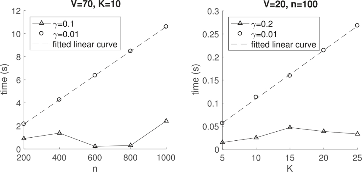
Average computation time (in seconds) per iteration of Algorithm 1 for 30 runs versus the number of graphs n (left) and rank K (right).
Fig. 2.
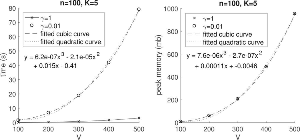
Average computation time (in seconds) per iteration (left) and average peak memory (in mb) in use (right) during the execution of Algorithm 1 for 30 runs versus the number of nodes V. The equation of the fitted cubic curve is shown on either plot.
The right plot in Figure 2 shows that the peak memory during the execution of Algorithm 1 is a cubic order with V no matter what penalty factor is used. This is in accordance with the theoretical memory complexity of Algorithm 1, O(V3 + VK + nK), in Section IV. We do not show the peak memory of Algorithm 1 versus the number of observations n or the rank K here because the peak memory is dominated by the cubic term of V and does not vary much with n or K in these cases.
Algorithm 1 was coded in the Matlab (R2017a) programming environment using no C or FORTRAN code. It is likely that the computational time of Algorithm 1 would improve relative to lasso or tensor regression if such code were used, as each iteration of Algorithm 1 involves for-loops over the elements of component vectors which are particularly slow in Matlab.
B. Inference on Signal Subgraphs
In this experiment, we compare the performance of recovering true signal subgraphs among lasso, TN-PCA (model (1)), naive TR (model (2)–(3)), LRS (model (4)) and our proposed symmetric bilinear regression with L1 penalty (SBL).
We simulate a synthetic dataset consisting of 100 pairs of observations {(Wi, yi) : i = 1, . . . ,100} as follows. Each pair consists of a 20 × 20 adjacency matrix Wi and a scalar . Specifically, each network Wi is generated from a set of basis subgraphs with an individual loading vector as
| (21) |
where qh ∈ {0, 1}20 is a random binary vector with ‖qh‖0 = h + 1, h = 1, . . . ,10.
The loadings {λih} in (21) are generated independently from N(0, 1). Δi is a symmetric 20 × 20 noise matrix with each entry Δi[uv] ~ N(0, 0.12), u > v. This generating process produces dense networks with complex structure. Figure 3 visualizes the 10 basis subgraphs superimposed together.
Fig. 3.
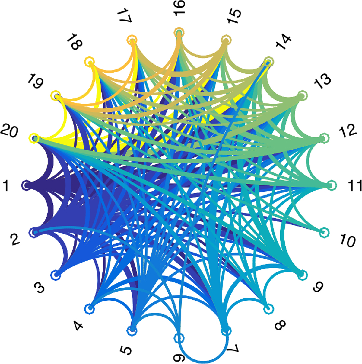
Overlay of 10 basis subgraphs corresponding to .
The response yi is generated by
| (22) |
where εi ~ N(0, σ2). We consider two noise levels: σ = 10% and 100% of the standard deviation of the conditional mean E(yi | Wi). The generating process (22) indicates that the true signal subgraphs relevant to yi correspond to the first three basis subgraphs as displayed in Figure 4, so that the true signal subgraphs have nontrivial variations across observations, as is often the case in practice.
Fig. 4.
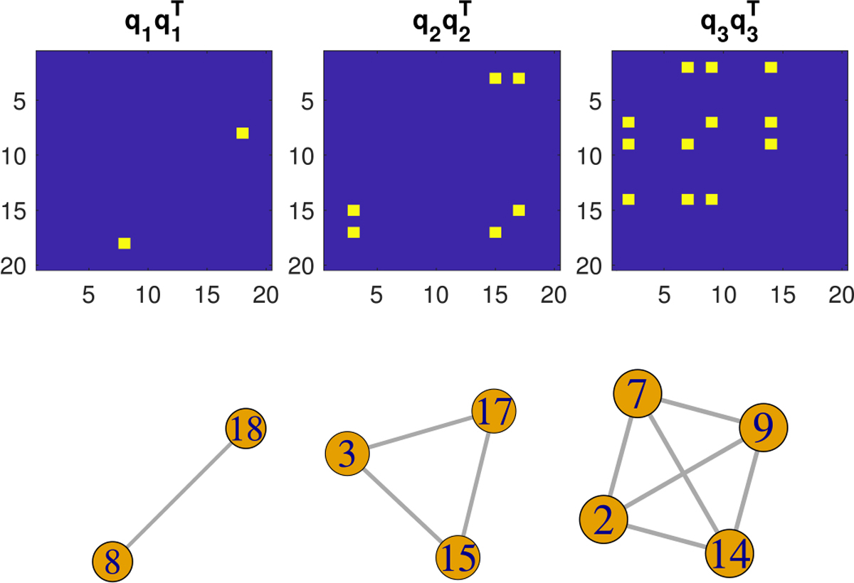
True signal subgraphs in simulation: (upper panel) and the corresponding clique subgraphs (lower panel).
1). High Signal-to-Noise Ratio:
In this case, we set the noise level σ = 10% of the standard deviation of the conditional mean E(yi | Wi) in the generating process (22).
The input parameters of Algorithm 1 for SBL are set as follows. K is set at 5 and the tolerance ϵ = 10−5 in this simulation study. It is easy to find a roughly smallest value γmax for which and become zero. We set γmin = 0.01γmax and choose a sequence of 50 equally spaced γ values on the logarithmic scale.
The dataset is split into a training set and a test set with each consisting of 50 observations, for tuning the L1 penalty factor. Figure 5 and 6 display the mean squared error (MSE) on test data across different values of the L1 penalty factor for lasso, naive TR and SBL respectively. As can be seen, the out-of-sample MSE does not vary much with small values of the penalty factor for each method. Therefore we set the optimal L1 penalty factor at the largest possible value that produces small MSE (e.g. less than 3% of the maximum MSE when all the parameters are zero in this case) for all models as indicated in Figure 5 and 6.
Fig. 5.
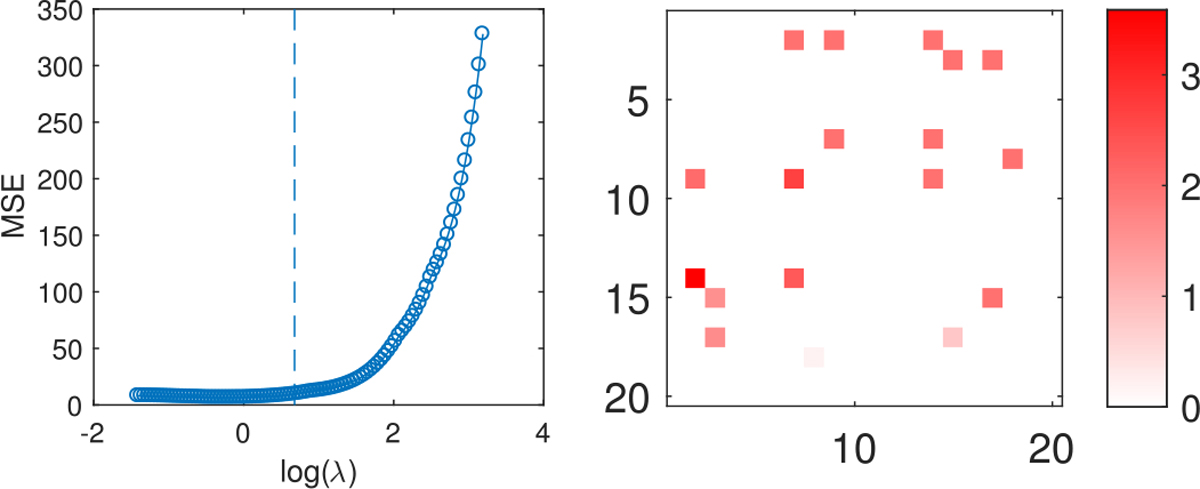
Left: out-of-sample MSE from lasso under high signal-to-noise ratio. Right: estimated coefficients from lasso (lower-triangular) where the L1 penalty factor is set corresponding to the vertical line on the left plot; the true coefficients for each edge of the network are shown in the upper triangle.
Fig. 6.

Out-of-sample MSE from naive TR (left) and SBL (right) under high signal-to-noise ratio. The vertical line in either plot indicates the selected value of the L1 penalty factor in coefficient estimation.
The estimated coefficients from lasso are displayed in the lower-triangular matrix in the right plot of Figure 5 with the true coefficients in the upper-triangular. As can be seen, lasso misses some true signal edges and it is not straightforward to identify meaningful structure among the selected edges.
For the linear regression based on TN-PCA, we set the rank K = 20 in (1), which explains approximately 100% of the variation in the networks. The MSE on test data from TN-PCA is 19.46, higher than the MSE at the optimal L1 penalty factor, 15.32 for naive TR, 9.67 for lasso and 9.17 for SBL. The linear regression on the network PC scores shows that all the 20 components are significant at the 5% significance level, which is noninformative of the subgraphs relevant to y since all the basis networks are dense.
For the low-rank sensing (LRS) model, we solve the optimization (4) by minimizing the nuclear norm [15] with the CVX toolbox in matlab. The solution for the coefficient matrix B does not have low rank but actually full rank in this case. This is probably due to the randomness in the generating process for y, which is closer to the reality in neuroimaging studies, while model (4) does not contain any randomness. In addition, the estimated B is a dense matrix with all the entries nonzero, and hence selects all the edges in the network. The MSE on test data from LRS is 13.46.
The estimated coefficient components for from SBL as well as the selected subgraphs are displayed in Figure 7, where 4 out of 5 components are nonempty. Figure 7 shows that our model recovers all the true signal subgraphs – a single edge, a triangle and a 4-node clique, though the component repeatedly selects an edge in the true triangle signal. Figure 8 displays the evolution of the estimated nonzero coefficients {λh βhu βhv} and 20 randomly selected zero coefficients in Figure 7 over iterations, which shows that the sequences of component coefficients converge as the objective function converges. In practice, we can always check such profiles of evolution for component coefficients and select a proper tolerance ϵ in Algorithm 1 to guarantee the convergence of solution sequences.
Fig. 7.
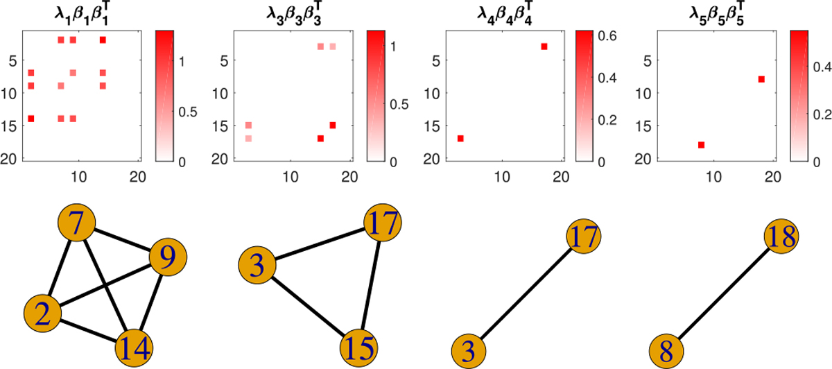
Estimated nonzero coefficient components from SBL (upper) and their selected subgraphs (lower) under high signal-to-noise ratio.
Fig. 8.
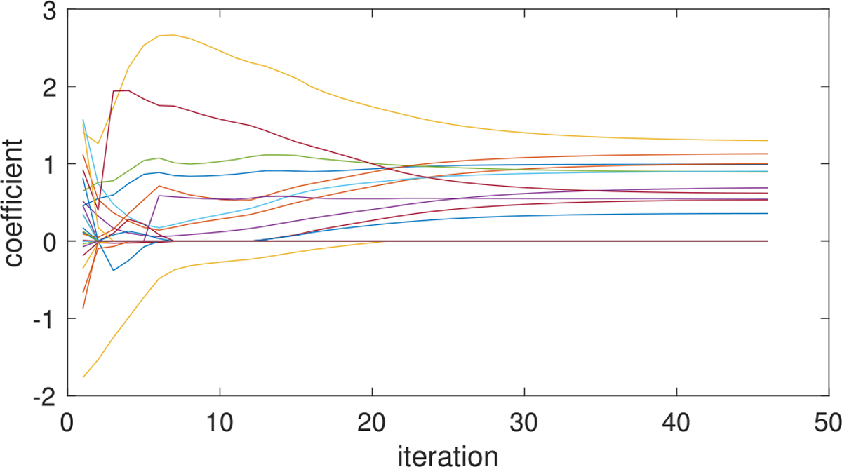
Profiles of estimated coefficients from SBL under high signal-to-noise ratio, showing how coefficient values {λh βhu βhv} evolve over iterations for the estimated nonzero coefficients and 20 randomly selected zero coefficients in Figure 7.
We use 10 initializations to run Algorithm 1 in this case, as the best local solution found does not change when increasing to 20 initializations. The total runtime is 32.2 seconds. But since the numerical experiments were conducted in a machine with one Intel Core i5 2.7 GHz processor and 8 GB of RAM, there are substantial margins to reduce the computational time if parallel computing were employed in a multi-core machine.
The naive TR is applied in this case under the same rank, the same convergence criterion and initializations as with SBL. The estimated coefficient components as well as the selected subgraphs are displayed in Figure 9, where 2 out of 5 components are nonempty. Figure 9 shows that the naive TR model partially recovers the 4-node clique and the triangle signal, though misses the single-edge signal.
Fig. 9.

Estimated nonzero coefficient components from naive TR and their selected subgraphs under high signal-to-noise ratio.
The procedure described above is repeated 100 times, where each time we generate a synthetic dataset based on (21) and (22), and record the out-of-sample MSE (at the optimal L1 penalty factor for lasso, naive TR and SBL), the true positive rate (TPR) representing the proportion of true signal edges that are correctly identified, and the false positive rate (FPR) representing the proportion of non-signal edges that are falsely identified, for lasso, TN-PCA, LRS, naive TR and SBL. Table II displays the mean and standard deviation (sd) of the MSE, TPR and FPR for the five methods in the high signal-to-noise ratio scenario. Although LRS has the lowest average MSE in Table II, its TPR and FPR are both 1, indicating that LRS selects all the edges in the network in each simulation. SBL has a bit higher average FPR than that of lasso and the highest TPR on average excluding LRS.
TABLE II.
Mean and SD of the MSE, TPR and FPR Across 100 Simulations Under High Signal-to-Noise Ratio
| MSE | TPR | FPR | |
|---|---|---|---|
|
| |||
| lasso | 10.98±4.40 | 0.837±0.138 | 0.002±0.005 |
| TN-PCA | 10.04±4.66 | 0.449±0.499 | 0.449±0.499 |
| LRS | 6.71±2.86 | 1.000±0.000 | 1.000±0.000 |
| naive TR | 15.94±6.93 | 0.696±0.122 | 0.024±0.027 |
| SBL | 10.08±4.51 | 0.848±0.169 | 0.005±0.007 |
2). Low Signal-to-Noise Ratio:
In this case, the noise level σ = 100% of the standard deviation of the conditional mean E(yi | Wi) in the generating process (22).
Figure 10 and 11 display the MSE on test data versus the L1 penalty factor for lasso, naive TR and SBL respectively. We set the optimal L1 penalty factor for each model at the value that produces the minimum out-of-sample MSE as indicated in Figure 10 and 11.
Fig. 10.
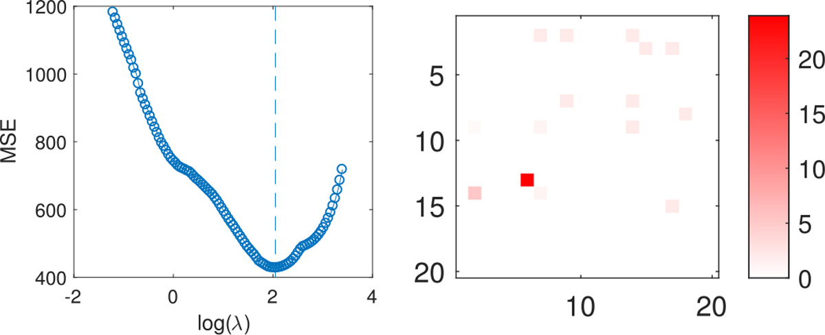
Left: out-of-sample MSE from lasso under low signal-to-noise ratio. Right: estimated coefficients from lasso (lower-triangular) where the L1 penalty factor is set corresponding to the vertical line on the left plot; the true coefficients for each edge of the network are shown in the upper triangle.
Fig. 11.
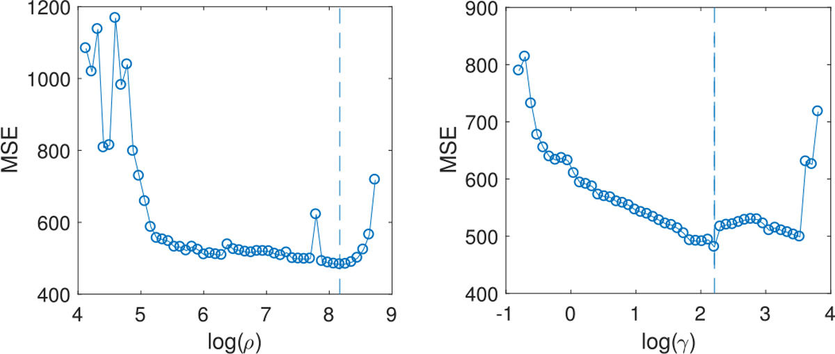
Out-of-sample MSE from naive TR (left) and SBL (right) under low signal-to-noise ratio. The vertical line in either plot indicates the selected value of the L1 penalty factor in coefficient estimation.
The estimated coefficients from lasso are displayed in the lower-triangular matrix in the left plot of Figure 10, which shows that lasso misses many true signal edges and selects a false edge with very large coefficient.
The MSE on test data from LRS is 1271.5 in this case and that from TN-PCA is 1249.1, much higher than the minimum MSE 482.8 for naive TR, 481.1 for SBL and 427.5 for lasso. The solution for coefficient matrix B from LRS is a dense matrix with full rank. The linear regression on the network PC scores from TN-PCA shows that none of the 20 components are significant in this case.
SBL selects two nonzero coefficient components out of 5 in this case, which are displayed in Figure 12 along with the selected subgraphs. Figure 12 shows that our model perfectly recovers one true signal subgraph – the 4-node clique, though partially recovers the triangle signal by identifying one edge and misses the single-edge signal. The evolution profiles of the estimated nonzero coefficients and 20 randomly selected zero coefficients in Figure 12 are displayed in Figure 13, which indicates the convergence of the coefficients. The total runtime under 10 initializations is 18 seconds in this case.
Fig. 12.

Estimated nonzero coefficient components from SBL and their selected subgraphs under low signal-to-noise ratio.
Fig. 13.
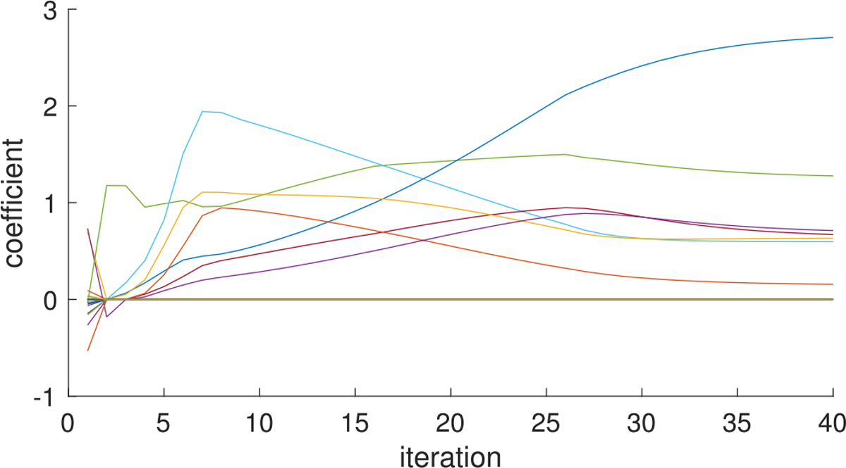
Profiles of estimated coefficients from SBL under low signal-to-noise ratio, showing how coefficient values {λh βhu βhv} evolve over iterations for the estimated nonzero coefficients and 20 randomly selected zero coefficients in Figure 12.
The naive TR is applied under the same convergence criterion and initializations as in SBL, where 1 out of 5 components is nonempty as displayed in Figure 14, which shows that the naive TR method partially recovers the 4-node clique while selecting 2 false edges.
Fig. 14.
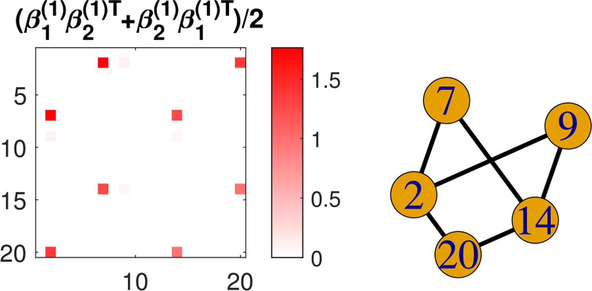
Estimated nonzero coefficient component from naive TR and its corresponding subgraph under low signal-to-noise ratio.
The procedure described above is again repeated 100 times and Table III displays the mean and sd of the out-of-sample MSE, TPR and FPR for the five methods in the low signal-to-noise ratio scenario. Table III shows that SBL has the lowest out-of-sample MSE on average. Although naive TR obtains a bit higher TPR on average than SBL in this case, it has much higher average FPR than that of lasso and SBL.
TABLE III.
Mean and SD of the MSE, TPR and FPR Across 100 Simulations Under Low Signal-to-Noise Ratio
| MSE | TPR | FPR | |
|---|---|---|---|
|
| |||
| lasso | 448.3±195.3 | 0.445±0.141 | 0.025±0.037 |
| TN-PCA | 624.0±287.8 | 0.060±0.239 | 0.060±0.238 |
| LRS | 636.7±258.3 | 1.000±0.000 | 1.000±0.000 |
| naive TR | 394.5±157.1 | 0.572±0.181 | 0.176±0.238 |
| SBL | 393.7±159.2 | 0.539±0.210 | 0.029±0.038 |
C. Sensitivity to K
In the experiments above, the rank K is set at 5 in SBL, which is an upper bound for the true rank of the generating process (22), as recommended in Section IV-D. To assess the sensitivity of SBL’s performance to the choice of K in practice, we rerun SBL with K = 6 and K = 7 for the experiments in both high and low signal-to-noise ratio (SNR) scenarios. The mean and sd of the out-of-sample MSE, TPR and FPR are displayed in Table IV. Compared to Table II and III in either case, the average MSEs, TPRs and FPRs are very similar among different choices for K in SBL, implying that Algorithm 1 is robust to the chosen upper bound for the rank.
TABLE IV.
Mean and SD of the MSE, TPR and FPR for SBL With Different Choices of K in High and Low Signal-to-Noise Ratio (SNR)
| MSE | TPR | FPR | ||
|---|---|---|---|---|
|
| ||||
| high | K = 6 | 10.21±4.62 | 0.856±0.182 | 0.004±0.011 |
| SNR | K = 7 | 10.15±4.61 | 0.858±0.172 | 0.005±0.009 |
|
| ||||
| low | K = 6 | 394.5±158.0 | 0.570±0.224 | 0.020±0.021 |
| SNR | K = 7 | 395.4±158.8 | 0.548±0.208 | 0.020±0.024 |
VI. Application
We applied our method to the Human Connectome Project (HCP) dataset [25], exploring the association between the brain connectome and two cognitive abilities, auditory language comprehension ability and oral reading ability. The dataset contains sMRI and dMRI data for 1065 subjects and for each subject, a weighted brain network of fiber counts among 68 regions was constructed by a state-of-the-art dMRI processing pipeline [26].
A. Picture Vocabulary Data
The HCP dataset contains age-adjusted scale scores of the subjects in a picture vocabulary (PV) test where respondents are presented with an audio recording of a word and four photographic images on the computer screen and are asked to select the picture that most closely matches the meaning of the word.
We first compare the predictive performance for the PV scores among lasso, TN-PCA and SBL. The dataset is partitioned into a training set of 565 subjects and a test set of 500 subjects. We set K = 10 for SBL. Five initializations are enough for Algorithm 1 to produce robust estimates for this dataset. The MSEs of PV scores on test data from SBL under different values of the L1 penalty factor γ are shown in Figure 15. The optimal γ is set at the value that produces the smallest MSE, which is smaller than the minimum MSE of lasso, indicating better predictive performance. We set the rank K = 68 in TN-PCA, which explains approximately 93% of the variation in the brain networks. The out-of-sample MSE of TN-PCA is 222.1, which is higher than the minimum MSE of SBL as indicated in Figure 15. The linear regression of the PV scores on the low-dimensional embeddings of the brain networks shows that none of the 68 components are significant at the 5% significance level.
Fig. 15.
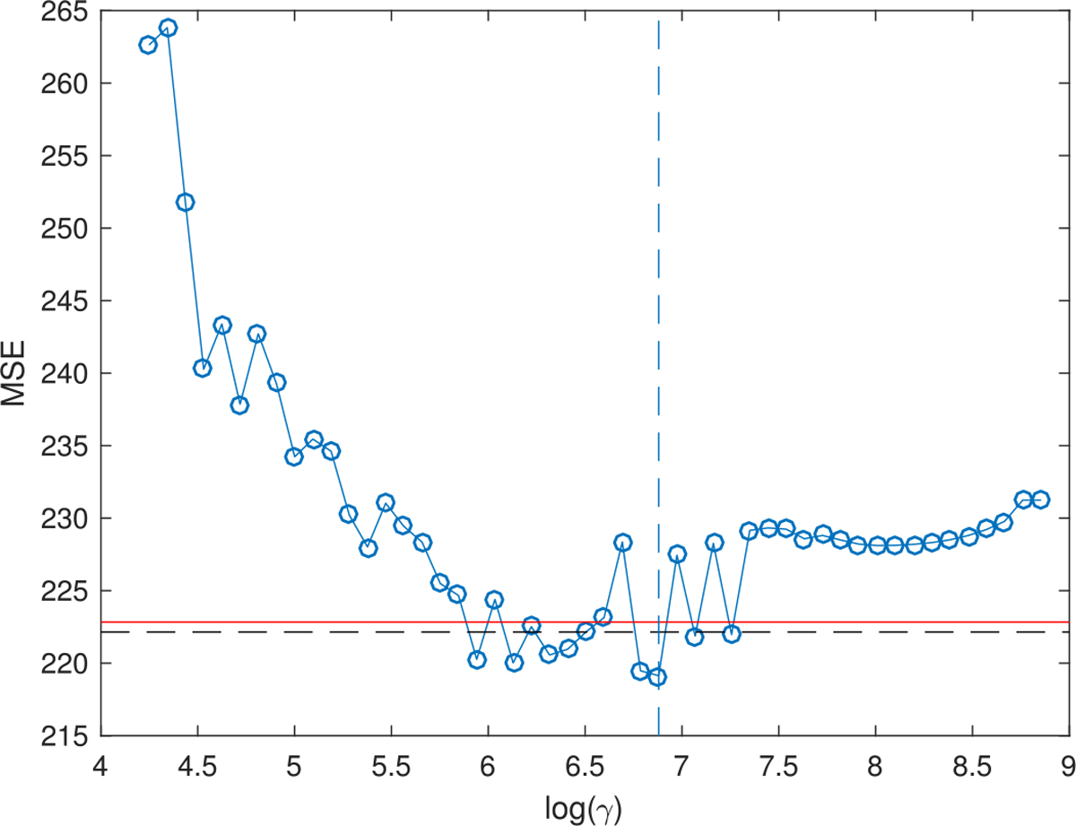
Out-of-sample MSE of SBL on picture vocabulary data. The dashed vertical line indicates the selected value of γ in inference; the red horizontal line indicates the minimum MSE of lasso; the black horizontal line indicates the MSE of TN-PCA.
The estimated coefficients from lasso and the structural connections in the brain corresponding to the nonzero coefficients are displayed in Figure 16. As can be seen, these identified connections lack meaningful structure and are difficult to justify neurologically.
Fig. 16.
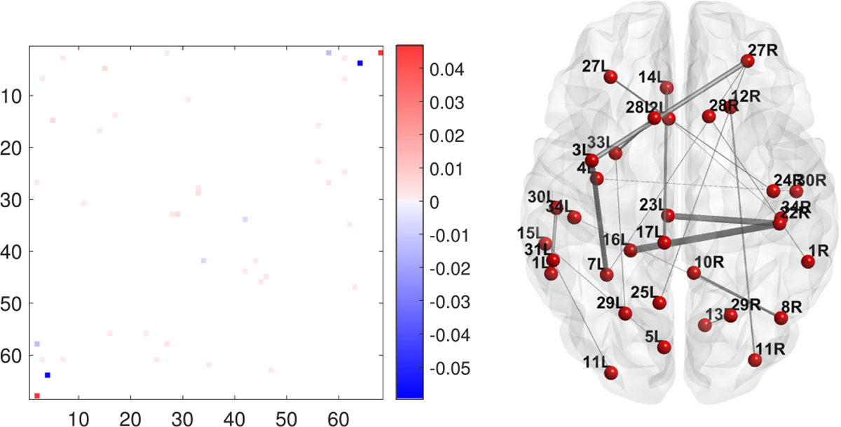
Estimated coefficients from lasso in matrix form (left) and the structural connections in the brain corresponding to nonzero coefficients (right). The thickness of each edge is proportional to the average fiber count between the pair of regions.
For L1-penalized symmetric bilinear regression, only 6 out of 10 coefficient component matrices have nonzero entries, implying K = 10 is large enough to capture all the signal subgraphs for this dataset. The estimated nonzero component matrices and their corresponding structural connections in the brain are displayed in Figure 17, which shows that SBL locates multiple simple subgraphs in the brain that may form some anatomical circuits in linguistic processing of sound to meaning. Three subgraphs in Figure 17 only contain a single connection verifying the flexibility of the model. We also observe that some brain regions repeatedly appear in the subgraphs in Figure 17, which may indicate important roles of these regions in auditory comprehension. For example, 27L, 27R (left and right superior frontal gyrus), 7L (left inferior parietal gyrus) and 29L (left superior temporal gyrus) are among activated regions when shifting from listening to meaningless pseudo sentences to listening to meaningful sentences [27], [28]. Figure 17 also shows that most estimated coefficients of the strengths of these signal connections are positive, implying that stronger neural connections among these regions are expected to lead to higher auditory comprehension ability. These identified anatomical subnetworks in the brain are consistent with the notion that auditory language processing is a complex process, which is the product of the coordinated activities of several brain regions.
Fig. 17.

Estimated nonzero component matrices for picture vocabulary data (upper) and their selected subgraphs in the brain (lower). The thickness of each edge is proportional to the average fiber count between the pair of brain regions.
B. Reading Recognition Data
The HCP dataset also contains the age-adjusted scale scores of the subjects in an oral reading recognition (RR) test where participants were scored on reading and pronouncing letters and words. We apply our method to find sub-networks in the brain connectome relevant to oral reading ability. Following the same procedure of partitioning data as in Section VI-A, we compare the predictive performance for the RR scores among lasso, TN-PCA and SBL. The minimum out-of-sample MSE of SBL is 201.8, which is smaller than that of lasso, 205.9. Although TN-PCA obtains the smallest MSE, 194.7, in this case, the resulting 16 significant components select all the connections in the brain network.
In this case, SBL selects 7 non-empty components out of 10 with penalty factor γ set at the optimal value. The subgraphs of brain connectome corresponding to these nonzero components are displayed in Figure 18. We notice that a triangle subgraph repeatedly appears in these subgraphs, consisting of three regions: 27L (left superior frontal), 23L (left precentral) and 22R (right posterior cingulate). This triangle subgraph may form a core anatomical circuit in the phonological reading pathway. These regions agree with the findings in neuroscience that the superior frontal gyrus is associated with word reading [29], left precentral gyrus is involved in phonological output [30] and the posterior cingulate cortex is associated with language comprehension [31].
Fig. 18.
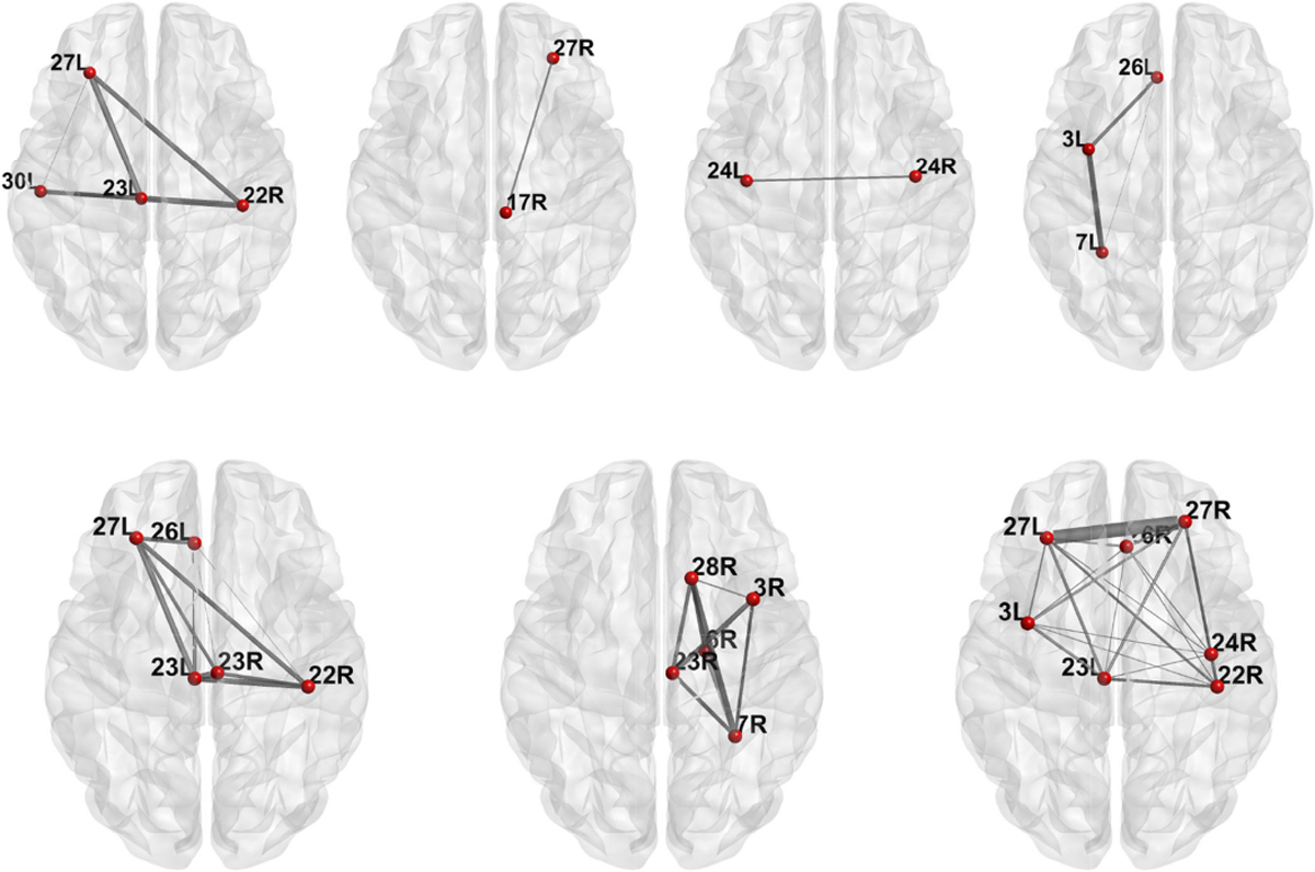
The selected subgraphs in the brain relevant to oral reading ability. The thickness of each edge is proportional to the average fiber count between the pair of brain regions.
VII. Conclusion
In summary, the symmetric bilinear model is a useful tool in analyzing the relationship between an outcome and a network-predictor, which produces much more interpretable results than unstructured regression does, while maintaining competitive predictive performance. We develop an effective coordinate descent algorithm for L1-penalized symmetric bilinear regression which outputs a set of small outcome-relevant subgraphs. Our method contributes to an insightful understanding of the substructure of networks that is relevant to the response and has wide applications in various fields such as neuroscience, internet mapping and social networks. Although we have focused on a continuous response, the methods are straightforward to adapt to classification problems and count responses by a simple modification of the goodness-of-fit component of the loss function.
Acknowledgment
Matlab code associated with this article can be found at https://doi.org/10.24433/CO.69bf9b86-3276-40fa-a979-b68a6ff1e562.
The associate editor coordinating the review of this manuscript and approving it for publication was Prof. Jarvis Haupt. This work was supported by Army Research Institute under Grant W911NF-16-1-0544.
Biographies

Lu Wang received the Ph.D. degree in statistics from Duke University, Durham, NC, USA, in May 2018. She is currently an Assistant Professor with the Department of Statistics, Central South University, Changsha, China. Her research interests include network analysis, Bayesian modeling, and high-dimensional optimization.

Zhengwu Zhang received the Ph.D. degree in statistics from Florida State University, Tallahassee, FL, USA, in May 2015. He is currently an Assistant Professor with the Department of Biostatistics and Computational Biology, University of Rochester, Rochester, NY, USA. His research interests include statistical image analysis, statistical shape analysis, Bayesian statistics, network analysis, and computational neuroscience.

David Dunson is the Arts and Sciences Distinguished Professor of statistical science, mathematics, and electronics and communication engineering with Duke University, Durham, NC, USA. He has made broad contributions in Bayesian statistical and signal processing methodology for complex and high-dimensional data, with a particular emphasis on nonparametric Bayesian approaches, dimensional reduction, and object data analysis. His methodology work is often directly motivated by and applied to data from scientific studies, with a particular focus on environmental health, genomics, and neuroscience. He is a Fellow of the American Statistical Association, Institute of Mathematical Statistics, and International Society for Bayesian Analysis. He was the recipient of the 2010 COPSS President’s Award given annually to one top statistician internationally age 40 or under.
Contributor Information
Lu Wang, Department of Statistics, Central South University, Changsha 410083, China.
Zhengwu Zhang, Department of Biostatistics and Computational Biology, University of Rochester, Rochester, NY 14604 USA.
David Dunson, Department of Statistical Science, Duke University, Durham, NC 27708 USA.
References
- [1].Tibshirani R, “Regression shrinkage and selection via the Lasso,” J. Roy. Statistical Soc. Ser. B (Methodological), vol. 58, no. 1, pp. 267–288, 1996. [Google Scholar]
- [2].Zou H and Hastie T, “Regularization and variable selection via the elastic net,” J. Roy. Statistical Soc. Ser. B (Statistical Methodology), vol. 67, no. 2, pp. 301–320, 2005. [Google Scholar]
- [3].Fan J and Li R, “Variable selection via nonconcave penalized likelihood and its oracle properties,” J. Amer. Statistical Assoc., vol. 96, no. 456, pp. 1348–1360, 2001. [Google Scholar]
- [4].Zheng D, Mhembere D, Burns R, Vogelstein J, Priebe CE, and Szalay AS, “Flashgraph: Processing billion-node graphs on an array of commodity SSDS,” in Proc. 13th USENIX Conf. File Storage Technologies, 2015, pp. 45–58. [Google Scholar]
- [5].Friedman J, Hastie T, and Tibshirani R, “Sparse inverse covariance estimation with the graphical Lasso,” Biostatistics, vol. 9, no. 3, pp. 432–441, 2008. [DOI] [PMC free article] [PubMed] [Google Scholar]
- [6].Beckmann CF, DeLuca M, Devlin JT, and Smith SM, “Investigations into resting-state connectivity using independent component analysis,” Philos. Trans. Roy. Soc. B, Biol. Sci., vol. 360, no. 1457, pp. 1001–1013, 2005. [DOI] [PMC free article] [PubMed] [Google Scholar]
- [7].Kolda TG and Bader BW, “Tensor decompositions and applications,” SIAM Rev., vol. 51, no. 3, pp. 455–500, 2009. [Google Scholar]
- [8].Varoquaux G, Gramfort A, Pedregosa F, Michel V, and Thirion B, “Multi-subject dictionary learning to segment an atlas of brain spontaneous activity,” in Proc. Biennial Int. Conf. Inf. Process. Med. Imag., 2011, pp. 562–573. [DOI] [PubMed] [Google Scholar]
- [9].Wang L, Zhang Z, and Dunson D, “Common and individual structure of brain networks,” 2017, arXiv:1707.06360. [Google Scholar]
- [10].Zhang Z, Allen G, Zhu H, and Dunson D, “Relationships between human brain structural connectomes and traits,” bioRxiv, 2018, Art. no. 256933. [DOI] [PMC free article] [PubMed] [Google Scholar]
- [11].Zhou H, Li L, and Zhu H, “Tensor regression with applications in neuroimaging data analysis,” J. Amer. Statistical Assoc., vol. 108, no. 502, pp. 540–552, 2013. [DOI] [PMC free article] [PubMed] [Google Scholar]
- [12].Zhou H and Li L, “Regularized matrix regression,” J. Roy. Statistical Soc. Ser. B (Statistical Methodology), vol. 76, no. 2, pp. 463–483, 2014. [DOI] [PMC free article] [PubMed] [Google Scholar]
- [13].Hoff PD, “Multilinear tensor regression for longitudinal relational data,” Ann. Appl. Statist., vol. 9, no. 3, pp. 1169–1193, 2015. [DOI] [PMC free article] [PubMed] [Google Scholar]
- [14].Li Z, Suk H-I, Shen D, and Li L, “Sparse multi-response tensor regression for Alzheimer’s disease study with multivariate clinical assessments,” IEEE Trans. Med. Imag., vol. 35, no. 8, pp. 1927–1936, Aug. 2016. [DOI] [PMC free article] [PubMed] [Google Scholar]
- [15].Recht B, Fazel M, and Parrilo PA, “Guaranteed minimum-rank solutions of linear matrix equations via nuclear norm minimization,” SIAM Rev., vol. 52, no. 3, pp. 471–501, 2010. [Google Scholar]
- [16].Jain P, Netrapalli P, and Sanghavi S, “Low-rank matrix completion using alternating minimization,” in Proc. 45th Annu. ACM Symp. Theory Comput., 2013, pp. 665–674. [Google Scholar]
- [17].Friedman J, Hastie T, and Tibshirani R, “Regularization paths for generalized linear models via coordinate descent,” J. Statistical Softw., vol. 33, no. 1, pp. 1–22, 2010. [PMC free article] [PubMed] [Google Scholar]
- [18].Sidiropoulos ND and Bro R, “On the uniqueness of multilinear decomposition of n-way arrays,” J. Chemometrics, vol. 14, no. 3, pp. 229–239, 2000. [Google Scholar]
- [19].Liu X and Sidiropoulos ND, “Cramér-Rao lower bounds for low-rank decomposition of multidimensional arrays,” IEEE Trans. Signal Process., vol. 49, no. 9, pp. 2074–2086, Sep. 2001. [Google Scholar]
- [20].de Lathauwer L, “A link between the canonical decomposition in multilinear algebra and simultaneous matrix diagonalization,” SIAM J. Matrix Anal. Appl., vol. 28, no. 3, pp. 642–666, 2006. [Google Scholar]
- [21].Allen G, “Sparse higher-order principal components analysis,” in Proc. 15th Int. Conf. Artif. Intell. Statist., 2012, pp. 27–36. [Google Scholar]
- [22].Schmidt M, “Least squares optimization with l1-norm regularization,” Univ. British Columbia, Tech. Rep. CS542B, 2005. [Google Scholar]
- [23].Ruszczyński AP, Nonlinear Optimization, vol. 13. Princeton, NJ, USA: Princeton Univ. Press, 2006. [Google Scholar]
- [24].Friedman J et al. , “Pathwise coordinate optimization,” Ann. Appl. Statist., vol. 1, no. 2, pp. 302–332, 2007. [Google Scholar]
- [25].van Essen DC et al. , “The human connectome project: A data acquisition perspective,” Neuroimage, vol. 62, no. 4, pp. 2222–2231, 2012. [DOI] [PMC free article] [PubMed] [Google Scholar]
- [26].Zhang Z et al. , “Mapping population-based structural connectomes,” NeuroImage, vol. 172, pp. 130–145, 2018. [DOI] [PMC free article] [PubMed] [Google Scholar]
- [27].Saur D et al. , “Ventral and dorsal pathways for language,” Proc. Nat. Acad. Sci., vol. 105, no. 46, pp. 18035–18040, 2008. [DOI] [PMC free article] [PubMed] [Google Scholar]
- [28].Dronkers NF, “The neural architecture of the language comprehension network: Converging evidence from lesion and connectivity analyses,” Frontiers Syst. Neuroscience, vol. 5, pp. 1–20, 2011. [DOI] [PMC free article] [PubMed] [Google Scholar]
- [29].Cloutman LL, Newhart M, Davis CL, Heidler-Gary J, and Hillis AE, “Neuroanatomical correlates of oral reading in acute left hemispheric stroke,” Brain Lang., vol. 116, no. 1, pp. 14–21, 2011. [DOI] [PMC free article] [PubMed] [Google Scholar]
- [30].Safi D et al. , “Recruitment of the left precentral gyrus in reading epilepsy: A multimodal neuroimaging study,” Epilepsy Behav. Case Rep., vol. 5, pp. 19–22, 2016. [DOI] [PMC free article] [PubMed] [Google Scholar]
- [31].Smallwood J et al. , “The default modes of reading: Modulation of posterior cingulate and medial prefrontal cortex connectivity associated with comprehension and task focus while reading,” Frontiers Human Neuroscience, vol. 7, pp. 734–743, 2013. [DOI] [PMC free article] [PubMed] [Google Scholar]


