


Figure 1.
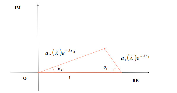
1, a1(λ)e−λτ1 and a2(λ)e−λτ2 form a triangle in the complex plane.
The time delay may induce oscillatory behaviour in multi-agent systems, which may destroy the consensus of the system. Therefore, the critical delay that is the maximum value of the delay to guarantee the consensus of the system, is an important performance index of multi-agent systems. This paper studies the influence of the processing delay on the consensus for a class of multi-agent system involving task strategies. The first-order system with a single delay and the second-order system with two different delays are investigated respectively. A critical delay independent of strategies and a critical region of the 2-D plane that depends on strategies is obtained for the first-order and the second-order system respectively. Specifically, a geometric method was used for the case of two different delays. Several numerical simulations are presented to explain the results.
Citation: Yipeng Chen, Yicheng Liu, Xiao Wang. The critical delay of the consensus for a class of multi-agent system involving task strategies[J]. Networks and Heterogeneous Media, 2023, 18(2): 513-531. doi: 10.3934/nhm.2023021
| [1] | Wenlian Lu, Fatihcan M. Atay, Jürgen Jost . Consensus and synchronization in discrete-time networks of multi-agents with stochastically switching topologies and time delays. Networks and Heterogeneous Media, 2011, 6(2): 329-349. doi: 10.3934/nhm.2011.6.329 |
| [2] | Yilun Shang . Group pinning consensus under fixed and randomly switching topologies with acyclic partition. Networks and Heterogeneous Media, 2014, 9(3): 553-573. doi: 10.3934/nhm.2014.9.553 |
| [3] | Yicheng Liu, Yipeng Chen, Jun Wu, Xiao Wang . Periodic consensus in network systems with general distributed processing delays. Networks and Heterogeneous Media, 2021, 16(1): 139-153. doi: 10.3934/nhm.2021002 |
| [4] | Yuntian Zhang, Xiaoliang Chen, Zexia Huang, Xianyong Li, Yajun Du . Managing consensus based on community classification in opinion dynamics. Networks and Heterogeneous Media, 2023, 18(2): 813-841. doi: 10.3934/nhm.2023035 |
| [5] | Mattia Bongini, Massimo Fornasier, Oliver Junge, Benjamin Scharf . Sparse control of alignment models in high dimension. Networks and Heterogeneous Media, 2015, 10(3): 647-697. doi: 10.3934/nhm.2015.10.647 |
| [6] | Riccardo Bonetto, Hildeberto Jardón Kojakhmetov . Nonlinear diffusion on networks: Perturbations and consensus dynamics. Networks and Heterogeneous Media, 2024, 19(3): 1344-1380. doi: 10.3934/nhm.2024058 |
| [7] | GuanLin Li, Sebastien Motsch, Dylan Weber . Bounded confidence dynamics and graph control: Enforcing consensus. Networks and Heterogeneous Media, 2020, 15(3): 489-517. doi: 10.3934/nhm.2020028 |
| [8] | Jean-Pierre de la Croix, Magnus Egerstedt . Analyzing human-swarm interactions using control Lyapunov functions and optimal control. Networks and Heterogeneous Media, 2015, 10(3): 609-630. doi: 10.3934/nhm.2015.10.609 |
| [9] | Giulia Cavagnari, Antonio Marigonda, Benedetto Piccoli . Optimal synchronization problem for a multi-agent system. Networks and Heterogeneous Media, 2017, 12(2): 277-295. doi: 10.3934/nhm.2017012 |
| [10] | Giuseppe Toscani, Andrea Tosin, Mattia Zanella . Kinetic modelling of multiple interactions in socio-economic systems. Networks and Heterogeneous Media, 2020, 15(3): 519-542. doi: 10.3934/nhm.2020029 |
The time delay may induce oscillatory behaviour in multi-agent systems, which may destroy the consensus of the system. Therefore, the critical delay that is the maximum value of the delay to guarantee the consensus of the system, is an important performance index of multi-agent systems. This paper studies the influence of the processing delay on the consensus for a class of multi-agent system involving task strategies. The first-order system with a single delay and the second-order system with two different delays are investigated respectively. A critical delay independent of strategies and a critical region of the 2-D plane that depends on strategies is obtained for the first-order and the second-order system respectively. Specifically, a geometric method was used for the case of two different delays. Several numerical simulations are presented to explain the results.
With the development of artificial intelligence, multi-agent systems have attracted extensive attention of researchers in computer science, physics, biology, social science and control engineering. The design of multi-agent systems is greatly influenced by the collective behaviour of animals in nature, such as ant colony gathering, birds flocking and fish swarming. Generally, a multi-agent system consists of multiple independent autonomous or semi-autonomous agents interconnected through a communication network, with research focuses including consensus [1], flocking [2], swarming [3], collision avoiding [4,5], formation control [6,7] and event-triggered control [8,9] etc. Consensus describes the process of agents coordination which has important applications in opinion dynamics and engineering control, and has been thoroughly analysed yielding a number of conditions guaranteeing that the agents reach consensus in the past decade, see [10,11,12,13,14].
The early literature on consensus has mainly focused on the analysis of autonomous systems whose final state after reaching consensus depends only on the initial configuration of the system. However, the application of autonomous system is limited because it is inconvenient and inflexible to use the target state to design the initial configuration of the system when the system is required to reach a specified state. One type of intervention, adding external forces to the system to reach the desired target state, is applicable to a variety of real-world contexts, such as financial markets, public opinion and a team of UAVs, and has been prevalent in multi-agent systems. Further, such interventions usually only affect a subset of individuals in the system, resulting in the leader-follower structure of multi-agent systems [15,16,17].
In a multi-agent system with leader-follower structure, the leaders refer to the part of agents who master information about the target state (i.e., those affected by the intervention), and the rest of the agents in the system is called followers. Leaders should not only carry out the information communication among the agents in the system, but also track the target state, while followers only are required to join in the information communication. In most previous researches, the information communication and the target tracking were separated, and the strength of target tracking was assumed to be finite based on the actual situation that the external force is limited by energy, equipment and technology.
Different from the above studies, this paper focuses more on the agent performance than on the external force. Considering the limited ability of agents, we assume that each agent has a task strategy to properly allocate its limited energy for the information communication and the target tracking. The detail of the first-order multi-agent system involving task strategies αi∈[0,m](i=1,2,⋯,N), is as follows:
| ˙xi(t)=f(t)+αi(x0(t)−xi(t))+(m−αi)1NN∑j=1(xj(t)−xi(t)),i=1,2,⋯,N, | (1.1) |
where xi(t) is the position of the ith agent, x0(t) is the target state satisfying ˙x0(t)=f(t), t≥0, f(t)∈C([0,∞),R), m∈R+ represents the maximal strength of the information communication. For the ith agent, the strength of the information communication is m−αi and the strength of the target tracking is αi. If αi>0, the ith agent is a leader, otherwise a follower. α=∑iαi is called the total strength of the target tracking of the system. The concept of the above strategy was proposed by Piccoli et al. [18] in 2016. They considered strategies {αi}Ni=1 as controls and focused on finding optimal control strategies {αi}Ni=1 to minimize the cost 1N∑Ni=1‖xi(T)−x0(T)‖, where T>0 was the final time. The Eq (1.1) with the non-linear information communication was investigated in [19], and the sufficient conditions were proposed to guarantee that the system achieves consensus. In addition to the first-order system (1.1), this paper also focuses on the second-order multi-agent system involving task strategies, written as
| ¨xi(t)=g(t)+αi[γ(v0(t)−˙xi(t))+(1−γ)(x0(t)−xi(t))]+(m−αi)[γNN∑j=1(˙xj(t)−˙xi(t))+1−γNN∑j=1(xj(t)−xi(t))], | (1.2) |
where γ∈[0,1] is the weight coefficient of velocities information, which measures the proportion of the velocities information in the control. Then the weight coefficient of positions information is 1−γ. x0(t) is the target state satisfying ˙x0(t)=v0(t), ˙v0(t)=g(t), t≥0, g(t)∈C([0,∞),R). Then, we present the mathematical definition of the consensus of the system for Eqs (1.1) and (1.2).
Definition 1.1. Suppose {xi(t)}Ni=1 is a solution of the Eq (1.1), x0(t) is the target state satisfying ˙x0(t)=f(t), t≥0, f(t)∈C([0,∞),R). The Eq (1.1) is said to achieve consensus and reach the target state if and only if
| limt→∞|xi(t)−x0(t)|=0,i=1,2,⋯,N. |
Suppose {xi(t)}Ni=1 is a solution of the Eq (1.2), x0(t) is the target state satisfying ˙x0(t)=v0(t), ˙v0(t)=g(t), t≥0, g(t)∈C([0,∞),R). The Eq (1.2) is said to achieve consensus and reach the target state if and only if
| limt→∞|xi(t)−x0(t)|=0andlimt→∞|˙xi(t)−v0(t)|=0,i=1,2,⋯,N. |
The time delay is an important topic in the research of multi-agent systems and has been widely studied. The causes of the time delay can be divided into two types: information transmission delay and information processing delay. The transmission delay means that it takes time for agents to receive information from others limited by the speed of communication, see [20,21,22]. The processing delay, also known as the reaction delay, refers to the time required for devices to process information, see [23,24,25]. The effect of time delay on consensus formation of multi-agent systems is an issue that cannot be ignored. Olfsti-Saber and Murray [26] gave a sufficient condition of consensus for a first-order system with time delay on balanced graphs and showed that there exists a trade-off between the control gain and the critical delay. Yu et al. [27] obtained some necessary and sufficient conditions for second-order consensus on directed graphs. Ma et al. studied a second-order consensus system with unstable elements over undirected graphs and maximized the critical delay by optimizing parameters [28]. A first-order consensus system with unstable elements over directed graphs was investigated in [29] and maximal critical delay was achieved through solving a nonsmooth max-min problem. For other relevant literature, see [30,31,32].
In this paper, we study the effect of the processing delay on the consensus of the first-order system in Eq (1.1) and the second-order system in Eq (1.2), and analyse the relationship between the processing delay and the strategies. According to the stability of linear systems in the theory of functional differential equations, the system would achieve consensus by ensuring that roots of the characteristic equation of the system have negative real parts. The specific content of the conclusion of stability is written as:
Lemma 1.2. [33] For a linear functional equation ˙u(t)=Au(t−r)+Bu(t−s), where u(t)∈RN, A,B∈RN×N and r,s∈R+. Its characteristic equation is h(λ)=Det(λI−Ae−λr−Be−λs)=0. Define a=sup{Reλ:h(λ)=0}, if a<0, the zero solution of the equation is globally asymptotically stable.
The rest of this paper is organized as follows. In Section 2, the Eq (1.1) with a single delay is investigated. Using the continuous dependence of the equation on the processing delay, we obtain the critical delay τ∗ that ensures that the Eq (1.1) achieves consensus, show that the critical delay τ∗ of the Eq (1.1) is independent of the strategies αi. In Section 3, the Eq (1.2) with two different delays is investigated. Inspired by [34,35,36] and using the properties of plane geometry, we identify the critical region D in R2 that guarantees the system to achieve consensus, find that the shape of the critical region D is affected by the strategies αi. In Section 4, several numerical simulations are presented to explain our results. Finally, we give the conclusion and discussion in Section 5.
Adding the processing delay in the Eq (1.1) yields
| ˙xi(t)=f(t)+αi(x0(t−τ)−xi(t−τ))+(m−αi)1NN∑j=1(xj(t−τ)−xi(t−τ)). | (2.1) |
where τ∈R+ represents the time required for the system to process the information of positions. Next we will transform the consensus problem of the Eq (2.1) into the stability problem of a linear autonomous system with a single delay, which further becomes the problem of judging whether the roots of the characteristic equation have negative real parts. Set yi(t)=xi(t)−x0(t), then the above model reduces to
| ˙yi(t)=−αiyi(t−τ)+(m−αi)1NN∑j=1(yj(t−τ)−yi(t−τ)). |
Define
| Y(t)=(y1(t),y2(t),⋅⋅⋅,yN(t))T∈RNandΓ=[m−α1Nm−α1N⋯m−α1Nm−α2Nm−α2N⋯m−α2N⋮⋮⋱⋮m−αNNm−αNN⋯m−αNN], | (2.2) |
then rewrite the above equations in matrix form
| ˙Y(t)=−mY(t−τ)+ΓY(t−τ). |
Compute the eigenvalues of the matrix Γ
| |μI−Γ|=|μ−m−α1N−m−α1N⋯−m−α1N−m−α2Nμ−m−α2N⋯−m−α2N⋮⋮⋱⋮−m−αNN−m−αNN⋯μ−m−αNN|=|μ−(m−α1)−m−α1N⋯−m−α1Nμ−(m−α2)μ−m−α2N⋯−m−α2N⋮⋮⋱⋮μ−(m−αN)−m−αNN⋯μ−m−αNN|=|μ−(m−α1)−μN⋯−μNμ−(m−α2)μ−μN⋯−μN⋮⋮⋱⋮μ−(m−αN)−μN⋯μ−μN|=|μ−(m−α1)−μN⋯−μNα2−α1μ⋯0⋮⋮⋱⋮αN−α10⋯μ|=|μ−(m−N∑i=1αiN)0⋯0α2−α1μ⋯0⋮⋮⋱⋮αN−α10⋯μ|=μN−1[μ−(m−αN)]=0, |
where α=∑Ni=1αi. Note that rank(Γ)=1, hence the matrix Γ is similarly diagonalized, i.e., there exists a non-singular matrix P such that PΓP−1=J, where J=diag(m−αN,0,⋯,0). Let Z(t)=PY(t), then the equation becomes
| ˙Z(t)=−mZ(t−τ)+JZ(t−τ). |
The characteristic equation of the above system is
| h(λ)=(λ+me−λτ)N−1(λ+αNe−λτ)=0. | (2.3) |
Hence, applying Lemma 1.2 we know that the Eq (2.1) achieves consensus if all roots of the Eq (2.3) have negative real parts. Using the continuous dependence of the Eq (2.3) on the processing delay τ, we obtain the following result.
Theorem 2.1. Assume α>0. Let Λ=sup{Reλ:h(λ)=0}, then there exists a critical delay
| τ∗=π2m |
such that Λ<0, ∀0≤τ<τ∗.
Proof. Owing to m,αN,τ∈R, ¯h(−iω)=h(iω), ∀ω∈R, which means that if λ=iω is a root of Eq (2.3), then also λ=−iω is a root. Without loss of generality let h(iω)=0, ω∈R+, then we obtain
| iω+me−iωτ=0oriω+αNe−iωτ=0. |
From iω+me−iωτ=0 we have mcos(ωτ)=0 and ω=msin(ωτ). Adding the squares of the two equations yields ω=m, then we have τkm=π2m+kπm, k∈Z. Similarly, from iω+αNe−iωτ=0 we could obtain τkα=πN2α+kπNα, k∈Z. Define
| τ∗=min{τkm,τkα,k=0,1,⋯}=π2m. |
When τ=0,
| h(λ)=(λ+m)N−1(λ+αN)=0. |
By α>0, Λ<0 which indicates that all roots of the Eq (2.3) lie on the left half complex plane when τ=0. Since h(λ) is continuously dependent on τ, Λ is continuously dependent on τ. Therefore, as the increase of τ from 0 to ∞, some roots of the Eq (2.3) touch the imaginary axis of the complex plane for the first time when τ=τ∗. Then, we conclude that Λ<0 if 0≤τ<τ∗ and Λ=0 if τ=τ∗.
Remark 1. Theorem 2.1 shows that the critical delay of the Eq (2.1) has nothing to do with strategies αi, but only with the maximal strength m.
Remark 2. If Λ<0 when τ=0, then the existence of the critical delay τ∗ is equivalent to the existence of some roots of the Eq (2.3) crossing the imaginary axis of the complex plane as the increase of τ from 0 to ∞. If the critical delay τ∗ exists, then it is the value of the delay when these roots first touch the imaginary axis.
Different from the Eq (1.1), the Eq (1.2) has to process not only the information of positions but also the information of velocities, so there are two different processing delays in the system. Adding the processing delay in the Eq (1.2) yields
| ¨xi(t)=g(t)+αi[γ(v0(t−τ1)−˙xi(t−τ1))+(1−γ)(x0(t−τ2)−xi(t−τ2))]+(m−αi)[γNN∑j=1(˙xj(t−τ1)−˙xi(t−τ1))+1−γNN∑j=1(xj(t−τ2)−xi(t−τ2))], | (3.1) |
where τ1 and τ2 represent times required for the system to process the information of positions and velocities, respectively. Similarly, we will transform the consensus problem of the Eq (3.1) into the stability problem of a linear autonomous system with two different delay. Set yi(t)=xi(t)−x0(t), the above model is simplified as
| ¨yi(t)=−αi[γ˙yi(t−τ1)+(1−γ)yi(t−τ2)]+(m−αi)[γNN∑j=1(˙yj(t−τ1)−˙yi(t−τ1))+1−γNN∑j=1(yj(t−τ2)−yi(t−τ2))], |
Define Y(t) and Γ same as Eq (2.2), then rewrite the equations in matrix form
| ¨Y(t)=−mγ˙Y(t−τ1)+γΓ˙Y(t−τ1)−m(1−γ)Y(t−τ2)+(1−γ)ΓY(t−τ2). |
Let Z(t)=PY(t), then the above equation becomes
| ¨Z(t)=−mγ˙Z(t−τ1)+γJ˙Z(t−τ1)−m(1−γ)Z(t−τ2)+(1−γ)JZ(t−τ2). |
The characteristic equation of the above system is
| h(λ)=[λ2+γmλe−λτ1+(1−γ)me−λτ2]N−1[λ2+γαNλe−λτ1+(1−γ)αNe−λτ2]=0. | (3.2) |
Let Λ=sup{Reλ:h(λ)=0}. When τ1=τ2=0, we have
| h(λ)=[λ2+γmλ+(1−γ)m]N−1[λ2+γαNλ+(1−γ)αN]=0. |
If α>0, it's easy to verify that Λ<0. Next, we firstly consider three simple cases: (1) τ1>0 and τ2=0; (2) τ1=0 and τ2>0; (3) τ1=τ2>0.
Theorem 3.1. Assume α>0, 0<γ<1. If one of the following three cases holds:
(1)
| 0=τ2<τ1<τ∗1=π2(γm2+√(1−γ)m+γ2m24), |
(2)
| 0=τ1<τ2<τ∗2=mins∈{m,αN}arctan(γs√−γ2s22+√(1−γ)2s2+γ4s44)√−γ2s22+√(1−γ)2s2+γ4s44, |
(3)
| 0<τ1=τ2<τ∗=arctan(γ1−γ√γ2m22+√(1−γ)2m2+γ4m44)√γ2m22+√(1−γ)2m2+γ4m44. |
Then Λ<0.
Proof. Because the proofs of (1) and (2) are very similar to the proof of (3), we will just prove the case τ1=τ2=τ>0 here. Without loss of generality let h(iω)=0, ω∈R+, then we have
| (iω)2+iγmωe−iωτ+(1−γ)me−iωτ=0 | (3.3) |
or
| (iω)2+iγαNωe−iωτ+(1−γ)αNe−iωτ=0. | (3.4) |
According to the Eq (3.3) we obtain
| {ω2=γmωsin(ωτ)+(1−γ)mcos(ωτ),0=γmωcos(ωτ)−(1−γ)msin(ωτ). | (3.5) |
Adding the squares of the above two equations yields
| ω4=γ2m2ω2+(1−γ)2m2, |
then we have
| ω=√γ2m22+√(1−γ)2m2+γ4m44. |
On the other hand, the second equation of Eq (3.5) gives
| τ=arctan(γω1−γ)ω=arctan(γ1−γ√γ2m22+√(1−γ)2m2+γ4m44)√γ2m22+√(1−γ)2m2+γ4m44≜τm. |
In the same way, according to the Eq (3.4) we could obtain
| τ=arctan(γ1−γ√γ2α22N2+√(1−γ)2α2N2+γ4α44N4)√γ2α22N2+√(1−γ)2α2N2+γ4α44N4≜τα. |
The critical delay τ∗=min{τm,τα}, so we need to determine the monotonicity of the function
| J(s)=arctan(γ1−γ√γ2s22+√(1−γ)2s2+γ4s44)√γ2s22+√(1−γ)2s2+γ4s44. |
Because √γ2s22+√(1−γ)2s2+γ4s44 is monotonically increasing with respect to s and arctanξξ is monotonically decreasing with respect to ξ, J(s) is monotonically decreasing with respect to s. Hence, we conclude τ∗=τm.
Remark 3. For the case (2), we cannot determine the monotonicity of the function
| J(s)=arctan(γs√−γ2s22+√(1−γ)2s2+γ4s44)√−γ2s22+√(1−γ)2s2+γ4s44 |
with respect to s. Actually, the numerical curve of J(s) shows that J(s) is monotonically increasing with respect to s. In addition, we assume 0<γ<1 in Theorem 3.1. By simple calculation we could obtain that if γ=1, the critical delay of τ1 is π2m; If γ=0, the critical delay of τ2 is π√m.
In the following we consider the case τ1≠τ2. In this case, the method applied in Theorems 2.1 and 3.1 is no longer feasible because we cannot obtain an explicit expression of τ∗ by solving for ω. Now we use a geometric method to analyse the Eq (3.2). From Eq (3.2) we have
| λ2+γmλe−λτ1+(1−γ)me−λτ2=0 |
or
| λ2+γαNλe−λτ1+(1−γ)αNe−λτ2=0. |
Since λ=0 is not a root of the above equations, the deformations of the equations are
| 1+γmλe−λτ1+(1−γ)mλ2e−λτ2=0 | (3.6) |
and
| 1+γαNλe−λτ1+(1−γ)αNλ2e−λτ2=0. | (3.7) |
For the Eq (3.6), let a1(λ)=γmλ and a2(λ)=(1−γ)mλ2. Think of 1, a1(λ)e−λτ1 and a2(λ)e−λτ2 as three vectors in the complex plane C, then λ is a root of the Eq (3.6) if and only if the three vectors are connected head to tail to form a triangle in the complex plane (See Figure 1).
Therefore, we could use the triangle property to get the relationship between λ, τ1 and τ2, and try to obtain the critical delay.
Theorem 3.2. Assume α>0, 0<γ<1. Then there exists a connected region D⊆R+×R+ such that Λ<0, ∀(τ1,τ2)∈D. In addition, the connected region D and its boundary ∂D satisfy
| D1≜D⋂{(τ1,τ2)|τ1∈R+,τ2=0}=[0,τ∗1)×{0}, |
| D2≜D⋂{(τ1,τ2)|τ1=0,τ2∈R+}={0}×[0,τ∗2), |
| D1∪D2∪{(τ∗,τ∗)}⊆∂Dand∂D∖(D1∪D2)⊆Φ∪Ψ, |
where
| Φ={(τ1,τ2)∈R+×R+|τ1=3π2+(2u−1)π±θ1ω,τ2=π+(2v−1)π∓θ2ω,u=u±0,u±0+1,⋯,v=v∓0,v∓0+1,⋯,ω∈Ω}, |
| Ψ={(τ1,τ2)∈R+×R+|τ1=3π2+(2p−1)π±ϑ1ω,τ2=π+(2q−1)π∓ϑ2ω,p=p±0,p±0+1,⋯,q=q∓0,q∓0+1,⋯,ω∈Υ}, |
τ∗1, τ∗2 and τ∗ are defined in Theorem 3.1, θ1, θ2, u±0, v∓0, Ω, ϑ1, ϑ2, p±0, q∓0 and Υ are defined in the proof.
Proof. The proof is divided into three steps.
The first step: use the triangle inequality to obtain the range of ω such that h(iω)=0. Without loss of generality let λ=iω, ω∈R+, then from Eq (3.6) we have
| 1+a1(iω)e−iωτ1+a2(iω)e−iωτ2=0, |
where a1(iω)=−γmωi and a2(iω)=−(1−γ)mω2. According to the triangle inequality that the length of any one side does not exceed the sum of the other two sides, we obtain
| |a1(iω)|+|a2(iω)|≥1,−1≤|a1(iω)|−|a2(iω)|≤1, |
i.e.
| ω2−γmω−(1−γ)m≤0,ω2−γmω+(1−γ)m≥0,ω2+γmω−(1−γ)m≥0. |
Denoting the range of ω by Ω and solving the inequalities yields
| Ω={[−γm2+√γ2m24+(1−γ)m,γm2+√γ2m24+(1−γ)m],4(1−γ)γ2≥m,[−γm2+√γ2m24+(1−γ)m,γm2−√γ2m24−(1−γ)m]∪[γm2+√γ2m24−(1−γ)m,γm2+√γ2m24+(1−γ)m],4(1−γ)γ2<m. |
Ω contains all the values of ω that make the roots of the Eq (3.6) lie on the imaginary axis of the complex plane at iω.
The second step: use Ω to calculate all the values of (τ1,τ2)∈R+×R+ that make h(iω)=0. Define ∡a1(iω)∈[0,2π) is the angle between a1(iω) with the positive direction of the real axis, θ1∈[0,π] is the inner angle of the triangle formed by a1(iω)e−iωτ1 and 1. Similar definitions apply to ∡a2(iω)∈[0,2π) and θ2∈[0,π]. Because a1(iω)=−γmωi and a2(iω)=−(1−γ)mω2, ∡a1(iω)=3π2 and ∡a2(iω)=π. By the law of cosine we have
| θ1=arccos(1+|a1(iω)|2−|a2(iω)|22|a1(iω)|)=arccos(ω2γm+γm2ω−(1−γ)2m2γω3), |
| θ2=arccos(1+|a2(iω)|2−|a1(iω)|22|a2(iω)|)=arccos(ω22(1−γ)m+(1−γ)m2ω2−γ2m2(1−γ)). |
Using properties of plane geometry we know that the angle between a1(iω)e−iωτ1 with the positive direction of the real axis plus or minus θ1 is equal to π, where plus or minus depends on whether the triangle is above or below the real axis. Similar results apply to a2(iω)e−iωτ2 and θ2. Then, we could establish the relations between τ1 with ω and τ2 with ω respectively:
| −ωτ1+2uπ+∡a1(iω)±θ1=π,u∈Z, |
| −ωτ2+2vπ+∡a2(iω)∓θ2=π,v∈Z, |
where −ωτ1+2uπ∈[0,2π) is the angle between e−iωτ1 with the positive direction of the real axis, −ωτ2+2vπ∈[0,2π) is the angle between e−iωτ2 with the positive direction of the real axis. Define u±0 and v∓0 are the smallest positive integers to guarantee τ1>0 and τ2>0 respectively, then we obtain
| τ1=∡a1(iω)+(2u−1)π±θ1ω=3π2+(2u−1)π±θ1ω,u=u±0,u±0+1,⋯, |
| τ2=∡a2(iω)+(2v−1)π∓θ2ω=π+(2v−1)π∓θ2ω,v=v∓0,v∓0+1,⋯. |
Define
| Φ={(τ1,τ2)∈R+×R+|τ1=3π2+(2u−1)π±θ1ω,τ2=π+(2v−1)π∓θ2ω,u=u±0,u±0+1,⋯,v=v∓0,v∓0+1,⋯,ω∈Ω}, |
then Φ⊆R+×R+ contains all the values of (τ1,τ2)⊆R+×R+ that make the roots of the Eq (3.6) lie on the imaginary axis.
Repeating the above steps for the Eq (3.7) yields that the roots of the Eq (3.7) lie on the imaginary axis if and only if (τ1,τ2)∈Ψ, where
| Ψ={(τ1,τ2)∈R+×R+|τ1=3π2+(2p−1)π±ϑ1ω,τ2=π+(2q−1)π∓ϑ2ω,p=p±0,p±0+1,⋯,q=q∓0,q∓0+1,⋯,ω∈Υ}, |
| ϑ1=arccos(ωN2γα+γα2ωN−(1−γ)2α2γω3N), |
| ϑ2=arccos(ω2N2(1−γ)α+(1−γ)α2ω2N−γ2α2(1−γ)N), |
| Υ={[−γα2N+√γ2α24N2+(1−γ)αN,γα2N+√γ2α24N2+(1−γ)αN],4(1−γ)γ2≥αN,[−γα2N+√γ2α24N2+(1−γ)αN,γα2N−√γ2α24N2−(1−γ)αN]∪[γα2N+√γ2α24N2−(1−γ)αN,γα2N+√γ2α24N2+(1−γ)αN],4(1−γ)γ2<αN. |
Hence, we proved that some roots of the Eq (3.2) lie on the imaginary axis if and only if (τ1,τ2)∈Φ∪Ψ.
The third step: combine Theorem 3.1 and Φ∪Ψ to determine the connected region D. By the results in [35,37], Φ∪Ψ characterizes a series of continuous curves on R+×R+ and divides R+×R+ into a series of connected regions. Let D represent the connected region containing the origin (0,0), then Theorem 3.1 indicates that the connected region D and its boundary ∂D satisfy
| D1≜D⋂{(τ1,τ2)|τ1∈R+,τ2=0}=[0,τ∗1)×{0}, |
| D2≜D⋂{(τ1,τ2)|τ1=0,τ2∈R+}={0}×[0,τ∗2), |
| D1∪D2∪{(τ∗,τ∗)}⊆∂Dand∂D∖(D1∪D2)⊆Φ∪Ψ. |
Because Λ<0 when (τ1,τ2)=(0,0)∈D, Λ=0 when (τ1,τ2)∈Φ∪Ψ and Λ is continuously dependent on (τ1,τ2), we conclude that Λ<0, ∀(τ1,τ2)∈D.
The the connected region D in Theorem 3.2 satisfies D1∪D2∪{(τ∗,τ∗)}⊆∂D and ∂D∖(D1∪D2)⊆Φ∪Ψ. Define the closure of D as ¯D, then we have Λ<0, ∀(τ1,τ2)∈D and Λ=0, ∀(τ1,τ2)∈¯D∖D. Hence, we call the connected region D the critical region. However, Φ∪Ψ contains so many curves that we cannot imagine the approximate range of D. By further analysing Φ∪Ψ, we will show that the critical region D is contained in a bounded region.
Theorem 3.3. Assume D is the critical region in Theorem 3.2. There exists a bounded region D∗⊆R+×R+ satisfying ∂D∗⊆D1∪D2∪C1∪C2 and ¯D∗∖D∗⊆C1∪C2 such that D⊆D∗, where
| C1={(τ1,τ2)∈R+×R+|τ1=π2−θ1ω,τ2=θ2ω,ω∈Ω}⊆Φ, |
| C2={(τ1,τ2)∈R+×R+|τ1=π2−ϑ1ω,τ2=ϑ2ω,ω∈Υ}⊆Ψ. |
D1, D2, θ1, θ2, Ω, ϑ1, ϑ2, and Υ are defined in Theorem 3.2.
Proof. Set
| b1≜a1(iω)e−iωτ1=−iγmωe−iωτ1andb2≜a2(iω)e−iωτ2=−(1−γ)mω2e−iωτ2. |
If (τ1,τ2)=(0,0), then ∡b1=3π2, ∡b2=π and the positions of 1, b1 and b2 on the complex plane are shown in Figure 2 Case 1. In this case, the Eq (3.6) do not have imaginary roots so that 1, b1 and b2 do not form a triangle in the complex plane. From Theorem 3.2 we know that 1, b1 and b2 could form a triangle for any (τ1,τ2)∈Φ∪Ψ. Select curves C1 and C2 from Φ∪Ψ, where
| C1={(τ1,τ2)∈R+×R+|τ1=π2−θ1ω,τ2=θ2ω,ω∈Ω}⊆Φ, |
| C2={(τ1,τ2)∈R+×R+|τ1=π2−ϑ1ω,τ2=ϑ2ω,ω∈Υ}⊆Ψ. |
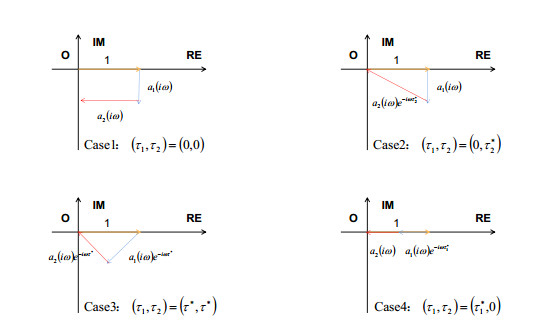
For the curve C1, let τ1=0 yields θ1=π2, then applying the properties of right triangle we obtain 1+|a1(iω)|2=|a2(iω)|2 and tan(θ2)=|a1(iω)|, (See Figure 2 Case 2) i.e.,
| 1+γ2m2ω2=(1−γ)2m2ω4andtan(θ2)=γmω. |
Solve the above equations yields
| ω=√−γ2m22+√(1−γ)2m2+γ4m44∈Ω,τ2=arctan(γmω)ω≥τ∗2. |
Let τ2=0 yields θ2=0, which means that the triangle degenerates into a line segment (See Figure 2 Case 4), so we have 1=|a1(iω)|+|a2(iω)| and θ1=0, and then
| ω=γm2+√γ2m24+(1−γ)m∈Ω,τ1=π2ω=τ∗1. |
Let τ1=τ2 yields θ1+θ2=π2, then we have 1=|a1(iω)|2+|a2(iω)|2 and tan(θ2)=|a1(iω)||a2(iω)| (See Figure 2 Case 3). By solving the above equation we obtain
| ω=√γ2m22+√(1−γ)2m2+γ4m44∈Ω,τ1=τ2=arctan(γω1−γ)ω=τ∗. |
Define a bounded region E1 formed by the curve C1 with the positive half of the horizontal and vertical axes, then the above statement indicates that D⊆E1. Similarly, For the curve C2, define a bounded region E2 formed by the curve C2 with the positive half of the horizontal and vertical axes, then we could verify that D⊆E2.
Let D∗=(E1∩E2)∖(C1∪C2), then D⊆D∗ and D is a bounded region. In addition, D∗ satisfies ∂D∗⊆D1∪D2∪C1∪C2 and ¯D∗∖D∗⊆C1∪C2.
Remark 4. Theorem 3.3 indicates that (τ∗1,0),(τ∗,τ∗)∈C1 and (0,τ∗2)∈C1∪C2. If curves in Φ∖C1 do not intersect the curve C1 and curves in Ψ∖C2 do not intersect the curve C2 (except at its endpoints), then D=D∗. In addition, unlike the Eq (2.1), Theorem 3.3 shows that the critical region D of the Eq (3.1) is related to both the total strength α and the maximal strength m.
In this section, a series of simulation examples are presented to illustrate Theorems 2.1, 3.1 and 3.3.
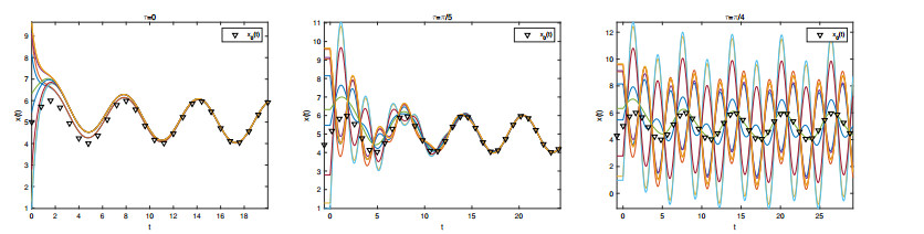
Set the target x0(t)=sin(t)+5 and f(t)=cos(t). Let N=10 and m=2, the initial positions xi(0) and strategies αi of the Eq (2.1) are listed in Table 1.
| x1(0)=8.1472 | x2(0)=9.0579 | x3(0)=1.2699 | x4(0)=9.1338 | x5(0)=6.3236 |
| α1=1 | α2=1 | α3=0 | α4=0 | α5=0 |
| x6(0)=0.9754 | x7(0)=2.7850 | x8(0)=5.4688 | x9(0)=9.5751 | x10(0)=9.6489 |
| α6=0 | α7=0 | α8=0 | α9=0 | α10=0 |
 DownLoad:
CSV
DownLoad:
CSV
According to Theorem 2.1, the critical delay τ∗=π2m=π4. Take τ=0, τ=π5 and τ=π4 respectively to obtain simulations of the Eq (2.1) as shown in Figure 3.
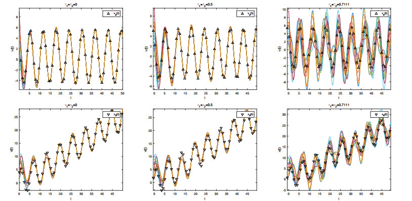
Set the target x0(t)=3sin(t)+4cos(t)+t2, v0(t)=3cos(t)−4sin(t)+12 and g(t)=−3sin(t)−4cos(t). Let N=10, m=2 and γ=0.5, the initial positions xi(0), velocities vi(t) and strategies αi of the Eq (3.1) are listed in Table 2.
| x1(0)=7.5127 | x2(0)=2.5510 | x3(0)=5.0596 | x4(0)=6.9908 | x5(0)=8.9090 |
| v1(0)=2.7603 | v2(0)=6.7970 | v3(0)=6.5510 | v4(0)=1.6261 | v5(0)=1.1900 |
| α1=1 | α2=1 | α3=0 | α4=0 | α5=0 |
| x6(0)=9.5929 | x7(0)=5.4722 | x8(0)=1.3862 | x9(0)=1.4929 | x10(0)=2.5751 |
| v6(0)=4.9836 | v7(0)=9.5976 | v8(0)=3.4039 | v9(0)=5.8527 | v10(0)=2.2381 |
| α6=0 | α7=0 | α8=0 | α9=0 | α10=0 |
DownLoad:
CSV
According to Theorem 3.1 we have τ∗1=π1+√5, τ∗2=min{1.1506,1.0166}=1.0166, τ∗=0.7111. Take τ1=τ2=0, τ1=τ2=0.5 and τ1=τ2=0.7111 respectively to obtain simulations of the Eq (3.1) as shown in Figure 4.
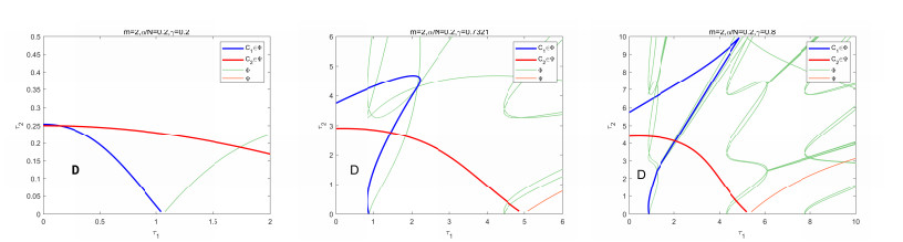
Fix m=2 and α/N=0.2, take γ=0.2, γ=0.7321 (i.e., 4(1−γ)γ2=m) and γ=0.8 respectively to obtain simulations of the Φ∪Ψ by Theorem 3.2, see Figure 5.
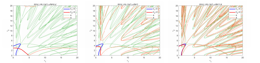
Fix m=2 and γ=0.7321, take α/N=0.2, α/N=1 and α/N=1.8 respectively to obtain simulations of the Φ∪Ψ by Theorem 3.2, see Figure 6.
In this paper, we analysed the influence of the processing delay on the consensus for the first-order system in Eq (1.1) and the second-order system in Eq (1.2). For the first-order system in Eq (2.1), by the continuous dependence of the equation on τ, we obtained the critical delay τ∗ that ensures the Eq (2.1) to achieve consensus and showed that the critical delay τ∗ is independent of the strategies αi. For the second-order system in Eq (3.1), from the properties of plane geometry, we identified the critical region D in R2 that guarantees the Eq (3.1) to achieve consensus and found that the shape of the critical region D is affected by the strategies αi.
The concept of strategies αi was firstly proposed by Piccoli et al. [18] to study the problem of optimal strategy. Using Pontryagin's minimum principle in optimal control theory, they found optimal strategies {αi}Ni=1 to minimize the cost 1N∑Ni=1‖xi(T)−x0(T)‖, where T>0 was the final time. More importantly, they showed that optimal strategies are sparse. From the present work, we want to find optimal strategies αi for the Eq (2.1) and analyse the influence of delays on the selection of optimal strategies αi.
We would like to thank the editors and the reviewers for their careful reading of the paper and their constructive comments.
This work was partially supported by the National Natural Science Foundation of China (11671011) and Hunan Provincial Innovation Foundation for Postgraduate (CN) (CX20220085).
The authors declare there is no conflict of interest.
| [1] |
R. Olfati-Saber, J. A. Fax, R. M. Murray, Consensus and cooperation in cetworked multi-Agent systems, Proc IEEE Inst Electr Electron Eng, 93 (2007), 215–233. https://doi.org/10.1016/j.lithos.2006.03.065 doi: 10.1016/j.lithos.2006.03.065

|
| [2] |
F. Cucker, S. Smale, Emergent behavior in flocks, IEEE Trans. Automat. Contr., 52 (2007), 852–862. https://doi.org/10.1109/TAC.2007.895842 doi: 10.1109/TAC.2007.895842
|
| [3] |
M. Brambilla, E. Ferrante, M. Birattari, M. Dorigo, Swarm robotics: a review from the swarm engineering perspective, Swarm Intell., 7 (2013), 1–41. https://doi.org/10.1007/s11721-012-0075-2 doi: 10.1007/s11721-012-0075-2
|
| [4] |
J. A. Carrillo, Y. P. Choi, P. B. Mucha, J. Peszek, Sharp condition to avoid collisions in singular Cucker-Smale interactions, Nonlinear Anal Real World Appl, 37 (2017), 317–328. https://doi.org/10.1016/j.nonrwa.2017.02.017 doi: 10.1016/j.nonrwa.2017.02.017
|
| [5] |
J. Hu, H. Zhang, L. Liu, X. Zhu, C. Zhao, Q. Pan, Convergent multiagent formation control with collision avoidance, IEEE Trans. Robot., 36 (2020), 1805–1818. https://doi.org/10.1109/TRO.2020.2998766 doi: 10.1109/TRO.2020.2998766
|
| [6] | K. K. Oh, M. C. Park, H. S. Ahn, A survey of multi-agent formation control, Automatica, 53 (2015), 424–440. |
| [7] |
Y. P. Choi, D. Kalise, J. Peszek, A. P. Andres, A Collisionless Singular Cucker-Smale model with decentralized formation control, SIAM J. Appl. Dyn. Syst., 18 (2019), 1954–1981. https://doi.org/10.1137/19M1241799 doi: 10.1137/19M1241799
|
| [8] |
D. V. Dimarogonas, E. Frazzoli, K. H. Johansson, Distributed event-triggered control for multi-agent systems, IEEE Trans. Automat. Contr., 57 (2012), 1291–1297. https://doi.org/10.1109/TAC.2011.2174666 doi: 10.1109/TAC.2011.2174666
|
| [9] |
X. Chen, H. Yu, F. Hao, Prescribed-time event-triggered bipartite consensus of multiagent systems, IEEE Trans Cybern, 52 (2022), 2589–2598. https://doi.org/10.1109/TCYB.2020.3004572 doi: 10.1109/TCYB.2020.3004572
|
| [10] |
Z. Li, G. Wen, Z. Duan, W. Ren, Designing fully distributed consensus protocols for linear multi-agent systems with directed graphs, IEEE Trans. Automat. Contr., 60 (2015), 1152–1157. https://doi.org/10.1109/TAC.2014.2350391 doi: 10.1109/TAC.2014.2350391
|
| [11] |
X. Jin, S. Lü, C. Deng, M. Chadli, Distributed adaptive security consensus control for a class of multi-agent systems under network decay and intermittent attacks, Inf. Sci., 547 (2021), 88–102. https://doi.org/10.1016/j.ins.2020.08.013 doi: 10.1016/j.ins.2020.08.013
|
| [12] |
S. Yu, X. Long, Finite-time consensus for second-order multi-agent systems with disturbances by integral sliding mode, Automatica, 54 (2015), 158–165. https://doi.org/10.1016/j.automatica.2015.02.001 doi: 10.1016/j.automatica.2015.02.001
|
| [13] |
H. Du, G. Wen, D. Wu, Y. Cheng, J. Lü, Distributed fixed-time consensus for nonlinear heterogeneous multi-agent systems, Automatica, 113 (2020), 108797. https://doi.org/10.1016/j.automatica.2019.108797 doi: 10.1016/j.automatica.2019.108797
|
| [14] |
J. Liu, Y. Zhang, Y. Yu, C. Sun, Fixed-time leader–follower consensus of networked nonlinear systems via event/self-triggered control, IEEE Trans Neural Netw Learn Syst, 31 (2020), 5029–5037. https://doi.org/10.1109/TNNLS.2019.2957069 doi: 10.1109/TNNLS.2019.2957069
|
| [15] |
Y. Hong, G. Chen, L. Bushnell, Distributed observers design for leader-following control of multi-agent networks, Automatica, 44 (2008), 846–850. https://doi.org/10.1016/j.automatica.2007.07.004 doi: 10.1016/j.automatica.2007.07.004
|
| [16] |
J. Shen, Cucker-Smale flocking under hierarchical leadership, SIAM J Appl Math, 68 (2008), 694–719. https://doi.org/10.1137/060673254 doi: 10.1137/060673254
|
| [17] |
J. Ni, P. Shi, Adaptive neural network fixed-time leader–follower consensus for multiagent systems with constraints and disturbances, IEEE Trans Cybern, 51 (2021), 1835–1848. https://doi.org/10.1109/TCYB.2020.2967995 doi: 10.1109/TCYB.2020.2967995
|
| [18] |
B. Piccoli, N. P. Duteil, B. Scharf, Optimal control of a collective migration model, Math Models Methods Appl Sci, 26 (2016), 383–417. https://doi.org/10.1142/S0218202516400066 doi: 10.1142/S0218202516400066
|
| [19] |
Y. Chen, Y. Liu, Flocking dynamics for a multiagent system involving task strategy, Math Models Methods Appl Sci, 46 (2023), 604–621. https://doi.org/10.1002/mma.8532 doi: 10.1002/mma.8532
|
| [20] | Y. Liu, J. Wu, Flocking and asymptotic velocity of the Cucker-Smale model with processing delay, J. Math. Anal. Appl., 415 (2014), 53-61. |
| [21] | Y. Liu, J. Wu, Opinion consensus with delay when the zero eigenvalue of the connection matrix is semi-simple, J Dyn Differ Equ, 29 (2016), 1–13. |
| [22] |
M. R. Cartabia, Cucker-Smale model with time delay, Discrete Contin Dyn Syst Ser A, 42 (2022), 2409–2432. https://doi.org/10.3934/dcds.2021195 doi: 10.3934/dcds.2021195
|
| [23] | X. Wang, L. Wang, J. Wu, Impacts of time delay on flocking dynamics of a two-agent flock model, Commun Nonlinear Sci Numer Simul, 70 (2019), 80–88. |
| [24] |
J. Haskovec, I. Markou, Asymptotic flocking in the Cucker-Smale model with reaction-type delays in the non-oscillatory regime, Kinet. Relat. Models, 13 (2020), 795–813. https://doi.org/10.3934/krm.2020027 doi: 10.3934/krm.2020027
|
| [25] |
Y. Liu, J. Wu, X. Wang, Collective periodic motions in a multiparticle model involving processing delay, Math. Methods Appl. Sci., 44 (2021), 3280–3302. https://doi.org/10.1002/mma.6939 doi: 10.1002/mma.6939
|
| [26] |
R. Olfsti-Saber, R. M. Murray, Consensus problem in networks of agents with switching topology and time-delays, IEEE Trans. Automat. Contr., 49 (2004), 1520–1533. https://doi.org/10.1109/TAC.2004.834113 doi: 10.1109/TAC.2004.834113
|
| [27] |
W. Yu, G. Chen, M. Cao, Some necessary and sufficient conditions for second-order consensus in multi-agent dynamical systems, Automatica, 46 (2010), 1089–1095. https://doi.org/10.1016/j.automatica.2010.03.006 doi: 10.1016/j.automatica.2010.03.006
|
| [28] |
D. Ma, R. Tian, A. Zulfiqar, J. Chen, T. Chai, Bounds on delay consensus margin of second-order multiagent systems with robust position and velocity feedback protocol, IEEE Trans. Automat. Contr., 64 (2019), 3780–3787. https://doi.org/10.1109/TAC.2018.2884154 doi: 10.1109/TAC.2018.2884154
|
| [29] | D. Ma, J. Chen, R. Lu, J. Chen, T. Chai, Delay effect on First-Order consensus over directed graphs: optimizing PID protocols for maximal robustness, SIAM J Control Optim, 60 (2022), 233–258. |
| [30] |
W. Yu, G. Chen, M. Cao, W. Ren, Delay-induced consensus and quasi-consensus in multi-agent dynamical systems, IEEE Trans Circuits Syst I Regul Pap, 60 (2013), 2679–2687. https://doi.org/10.1109/TCSI.2013.2244357 doi: 10.1109/TCSI.2013.2244357
|
| [31] |
W. Hou, M. Fu, H. Zhang, Z. Wu, Consensus conditions for general second-order multi-agent systems with communication delay, Automatica, 75 (2017), 293–298. https://doi.org/10.1016/j.automatica.2016.09.042 doi: 10.1016/j.automatica.2016.09.042
|
| [32] |
Q. Ma, S. Xu, Consensus switching of second-order multiagent systems with time delay, IEEE Trans Cybern, 52 (2022), 3349–3353. https://doi.org/10.1109/TCYB.2020.3011448 doi: 10.1109/TCYB.2020.3011448
|
| [33] | J. K. Hale, S. M. V. Lunel, Introduction to Functional Differential Equations, Berlin: Springer-Verlag, 1993. |
| [34] |
E. Beretta, Y. Kuang, Geometric stability switch criteria in delay differential systems with delay dependent parameters, SIAM J. Math. Anal., 33 (2002), 1144–1165. https://doi.org/10.1137/S0036141000376086 doi: 10.1137/S0036141000376086
|
| [35] | K. Gu, S. I. Niculescu, J. Chen, On stability crossing curves for general systems with two delays, J. Math. Anal. Appl., 331 (2005), 231–253. |
| [36] |
Q. Ma, S. Xu, Exact delay bounds of second-order multi-agent systems with input and communication delays, IEEE Trans. Circuits Syst. II Express Briefs, 69 (2022), 1119-1123. https://doi.org/10.1109/TCSII.2021.3094185 doi: 10.1109/TCSII.2021.3094185
|
| [37] |
L. hang, X. Li, Z. Mao, J. Chen, G. Fan, Some new algebraic and geometric analysis for local stability crossing curves, Automatica, 123 (2021), 109312. https://doi.org/10.1016/j.automatica.2020.109312 doi: 10.1016/j.automatica.2020.109312
|
| 1. | Fausto Francesco Lizzio, Elisa Capello, Yasumasa Fujisaki, Leader–Follower Formation of Second-Order Agents via Delayed Relative Displacement Feedback, 2023, 7, 2475-1456, 2335, 10.1109/LCSYS.2023.3285901 |
Figures(6) / Tables(2)
Yipeng Chen, Yicheng Liu, Xiao Wang. The critical delay of the consensus for a class of multi-agent system involving task strategies[J]. Networks and Heterogeneous Media, 2023, 18(2): 513-531. doi: 10.3934/nhm.2023021

| x1(0)=8.1472 | x2(0)=9.0579 | x3(0)=1.2699 | x4(0)=9.1338 | x5(0)=6.3236 |
| α1=1 | α2=1 | α3=0 | α4=0 | α5=0 |
| x6(0)=0.9754 | x7(0)=2.7850 | x8(0)=5.4688 | x9(0)=9.5751 | x10(0)=9.6489 |
| α6=0 | α7=0 | α8=0 | α9=0 | α10=0 |
DownLoad:
CSV
| x1(0)=7.5127 | x2(0)=2.5510 | x3(0)=5.0596 | x4(0)=6.9908 | x5(0)=8.9090 |
| v1(0)=2.7603 | v2(0)=6.7970 | v3(0)=6.5510 | v4(0)=1.6261 | v5(0)=1.1900 |
| α1=1 | α2=1 | α3=0 | α4=0 | α5=0 |
| x6(0)=9.5929 | x7(0)=5.4722 | x8(0)=1.3862 | x9(0)=1.4929 | x10(0)=2.5751 |
| v6(0)=4.9836 | v7(0)=9.5976 | v8(0)=3.4039 | v9(0)=5.8527 | v10(0)=2.2381 |
| α6=0 | α7=0 | α8=0 | α9=0 | α10=0 |
DownLoad:
CSV
| x1(0)=8.1472 | x2(0)=9.0579 | x3(0)=1.2699 | x4(0)=9.1338 | x5(0)=6.3236 |
| α1=1 | α2=1 | α3=0 | α4=0 | α5=0 |
| x6(0)=0.9754 | x7(0)=2.7850 | x8(0)=5.4688 | x9(0)=9.5751 | x10(0)=9.6489 |
| α6=0 | α7=0 | α8=0 | α9=0 | α10=0 |
| x1(0)=7.5127 | x2(0)=2.5510 | x3(0)=5.0596 | x4(0)=6.9908 | x5(0)=8.9090 |
| v1(0)=2.7603 | v2(0)=6.7970 | v3(0)=6.5510 | v4(0)=1.6261 | v5(0)=1.1900 |
| α1=1 | α2=1 | α3=0 | α4=0 | α5=0 |
| x6(0)=9.5929 | x7(0)=5.4722 | x8(0)=1.3862 | x9(0)=1.4929 | x10(0)=2.5751 |
| v6(0)=4.9836 | v7(0)=9.5976 | v8(0)=3.4039 | v9(0)=5.8527 | v10(0)=2.2381 |
| α6=0 | α7=0 | α8=0 | α9=0 | α10=0 |
