


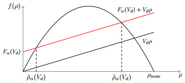
Figure 1.
The flux function f and ˇρα(V)⩽ˆρα(V)⩽ρ∗(V).
We consider a partial differential equation - ordinary differential equation system to describe the dynamics of traffic flow with autonomous vehicles. In the model, the bulk flow of human drivers is represented by a scalar conservation law, while each autonomous vehicle is described by an ordinary differential equation. The coupled PDE-ODE model is introduced, and existence of solutions for this model is shown, along with a proposed algorithm to construct approximate solutions. Next, we propose a control strategy for the speeds of the autonomous vehicles to minimize the average fuel consumption of the entire traffic flow. Existence of solutions for the optimal control problem is proved, and we numerically show that a reduction in average fuel consumption is possible with an AV acting as a moving bottleneck.
Citation: Thibault Liard, Raphael Stern, Maria Laura Delle Monache. A PDE-ODE model for traffic control with autonomous vehicles[J]. Networks and Heterogeneous Media, 2023, 18(3): 1190-1206. doi: 10.3934/nhm.2023051
| [1] | Paola Goatin, Chiara Daini, Maria Laura Delle Monache, Antonella Ferrara . Interacting moving bottlenecks in traffic flow. Networks and Heterogeneous Media, 2023, 18(2): 930-945. doi: 10.3934/nhm.2023040 |
| [2] | Abraham Sylla . Influence of a slow moving vehicle on traffic: Well-posedness and approximation for a mildly nonlocal model. Networks and Heterogeneous Media, 2021, 16(2): 221-256. doi: 10.3934/nhm.2021005 |
| [3] | Maya Briani, Rosanna Manzo, Benedetto Piccoli, Luigi Rarità . Estimation of NO$ _{x} $ and O$ _{3} $ reduction by dissipating traffic waves. Networks and Heterogeneous Media, 2024, 19(2): 822-841. doi: 10.3934/nhm.2024037 |
| [4] | Edward S. Canepa, Alexandre M. Bayen, Christian G. Claudel . Spoofing cyber attack detection in probe-based traffic monitoring systems using mixed integer linear programming. Networks and Heterogeneous Media, 2013, 8(3): 783-802. doi: 10.3934/nhm.2013.8.783 |
| [5] | Maria Teresa Chiri, Xiaoqian Gong, Benedetto Piccoli . Mean-field limit of a hybrid system for multi-lane car-truck traffic. Networks and Heterogeneous Media, 2023, 18(2): 723-752. doi: 10.3934/nhm.2023031 |
| [6] | Tong Li . Qualitative analysis of some PDE models of traffic flow. Networks and Heterogeneous Media, 2013, 8(3): 773-781. doi: 10.3934/nhm.2013.8.773 |
| [7] | F. A. Chiarello, J. Friedrich, S. Göttlich . A non-local traffic flow model for 1-to-1 junctions with buffer. Networks and Heterogeneous Media, 2024, 19(1): 405-429. doi: 10.3934/nhm.2024018 |
| [8] | Wen Shen . Traveling wave profiles for a Follow-the-Leader model for traffic flow with rough road condition. Networks and Heterogeneous Media, 2018, 13(3): 449-478. doi: 10.3934/nhm.2018020 |
| [9] | Florent Berthelin, Thierry Goudon, Bastien Polizzi, Magali Ribot . Asymptotic problems and numerical schemes for traffic flows with unilateral constraints describing the formation of jams. Networks and Heterogeneous Media, 2017, 12(4): 591-617. doi: 10.3934/nhm.2017024 |
| [10] | Maya Briani, Emiliano Cristiani . An easy-to-use algorithm for simulating traffic flow on networks: Theoretical study. Networks and Heterogeneous Media, 2014, 9(3): 519-552. doi: 10.3934/nhm.2014.9.519 |
We consider a partial differential equation - ordinary differential equation system to describe the dynamics of traffic flow with autonomous vehicles. In the model, the bulk flow of human drivers is represented by a scalar conservation law, while each autonomous vehicle is described by an ordinary differential equation. The coupled PDE-ODE model is introduced, and existence of solutions for this model is shown, along with a proposed algorithm to construct approximate solutions. Next, we propose a control strategy for the speeds of the autonomous vehicles to minimize the average fuel consumption of the entire traffic flow. Existence of solutions for the optimal control problem is proved, and we numerically show that a reduction in average fuel consumption is possible with an AV acting as a moving bottleneck.
The advent of vehicle automation has the potential to substantially transform the management of transportation systems. As disruptive technologies such as autonomous vehicles (AVs) come closer to reality, the potential for improved traffic control using AVs as Lagrangian actuators in the traffic flow has become a significant focus both theoretically [5,7,14,15,16,26,27] and experimentally [25].
Such control strategies rely on traffic models to capture the dynamics of the traffic flow. These models generally can be categorized as either microscopic or macroscopic, referring to the resolution at which the traffic is modeled. Microscopic traffic models use ordinary differential equations (ODEs) to model the dynamics of each individual vehicle in the traffic flow as a function of the local traffic state, while macroscopic traffic flow models use partial differential equations (PDEs) to model the evolution of traffic density on a roadway using conservation of mass (vehicles). While microscopic traffic flow models are able to capture the dynamics of each vehicle in the traffic flow, and allow for differentiation between individual vehicle dynamics, they can become computationally intractable at large scales. However, while computationally tractable at large scale, macroscopic models generally do not allow for differentiation between different vehicles with unique dynamics.
In the context of a relatively small number of AVs that may soon be present in the traffic flow navigating a bulk traffic that is made up primarily of human-piloted vehicles, the concept of coupled micro-macro models has been proposed [9]. The motivation behind such models is to use a PDE to model the density evolution of the primarily human-driven human traffic flow, and use a small number of ODEs to model the trajectories of AVs through that bulk traffic flow. These models are referred to as PDE-ODE or micro-macro models.
Recent results for weakly-coupled PDE-ODE systems, where the AV drives according to the local density solution of the PDE but does not locally constrain the flux of vehicles in the PDE, have shown that a fleet of such AVs can be used to estimate the traffic state between subsequent AVs [11]. Others have shown that by considering the strongly coupled PDE-ODE system where the presence of AVs locally acts as a moving bottleneck and restricts the traffic flux can be used for traffic control. In particular, one can look at Lagrangian control where a certain number of vehicles are controlled within the bulk traffic flow to act as bottlenecks. Recently, two seminal works [4,21] have proposed strategies to control traffic using such an approach. Both these works look to control traffic via means of autonomous vehicles: in [21], the Piacentini, et al. use a model predictive control (MPC) approach to achieve a reduction in fuel consumption in congested traffic; Čicic et al. [4] dissipate a traffic jam via the use of controlled autonomous vehicles.
We extend the existing work in [9] and consider the case of a fleet of multiple AVs acting as moving bottlenecks in the traffic flow. Each AV will be described by a different ODE and several flux constraints on the human-driven traffic PDE will be in place. We base our work on the results available for the micro-macro models of [9]. In particular, existence and well-posedness of solution were investigated in [10,18,19], the numerical aspects in [3,8] and the existence of controls were analyzed in [13]. Using those existing results, we are able to prove the existence of solution for the extended coupled PDE-ODE model. Using this extended model, we study the control problem of how to drive the AVs to achieve a certain traffic state to reduce the average fuel consumption of the overall traffic flow. The underlying idea is to exploit the dynamics of the AV by controlling it to drive according to a specific control law. In this way the interaction between the controlled vehicle and the surrounding flow can be used to modify the traffic density and improve congestion and reduce fuel consumption. We consider the speed of the moving bottleneck as the control variable when designing the control law, and use this for traffic control.
The remainder of this article is organized as follows: Section 2 presents the modeling framework and extends the framework to consider multiple AVs acting as moving bottlenecks in the flow while also presenting an analytical method to find solutions to the Riemann problem of PDE-ODE systems. In Section 2.3 we show how to compute approximate solutions to the coupled PDE-ODE system, and in Section 3 we introduce an optimal control problem and prove that this optimal control problem has at least one solution. Section 4 shows the numerical scheme and the simulations.
When modeling the evolution of the macroscopic traffic state, a common choice of conservation law used in traffic flow modeling is the Lighthill-Whitham-Richards (LWR) [20,23] PDE:
| ∂tρ(t,x)+∂xf(ρ(t,x))=0,t>0,x∈IR,ρ(0,x)=ρ0(x),x∈IR. | (2.1) |
where ρ=ρ(t,x)∈[0,ρmax] denotes the macroscopic traffic density at time t≥0 and position x∈IR, and f=f(ρ) is the density dependent flux function. The flux is given by f(ρ)=ρv(ρ) with v the mean speed of cars. In this paper we assume that the speed v depends linearly on the density of cars as follows:
| v(ρ)=Vmax(1−ρρmax), | (2.2) |
with constant maximal density ρmax and constant maximal speed Vmax.
Then, we assume that N controlled autonomous vehicles (AVs) are present on the road and their position is indicated by yi. The trajectory of the ith autonomous vehicle, for i∈{1,⋯,N}, is modeled by the following ODE
| ˙yi(t)=min{Vi(t),v(ρ(t,yi(t)+))},t>0,yi(0)=y0i. | (2.3) |
Above, Vi(t) is the control function, selecting the desired speed of the vehicle. The ith AV drives at its maximum desired speed Vi except when the traffic in front is too dense. In that case, the autonomous vehicle has to reduce its velocity accordingly. The notation ρ(t,yi(t)+) indicates the right trace of ρ with respect to the variable x, i.e., v(ρ(t,yi(t)+)):=limx→yi(t)x>yi(t)ρ(t,x). This allows us to assume that the autonomous vehicles are affected only by the downstream density.
To describe the influence of the ith AV on the evolution of traffic we introduce the following flux constraint:
| f(ρ(t,yi(t)))−˙yi(t)ρ(t,yi(t))≤Fα(˙yi(t)),t>0. | (2.4) |
The function Fα, α∈(0,1), models the maximal road capacity reduction due to the presence of the ith autonomous vehicle, that acts as a moving bottleneck which imposes unilateral constraints at the AVs positions. In accordance to [9], Fα, is defined as follows:
| Fα(˙yi(t)):=αmaxρ∈[0,ρmax](f(ρ)−˙yi(t)ρ). |
For simplicity of notation, in the rest of this section we drop the index i and use Vi and V interchangeably.
Thus, following the model proposed in [9], we model the impact of N∈IN∖{0} autonomous vehicles (AVs) on traffic flow via the following model:
| {∂tρ(t,x)+∂xf(ρ(t,x))=0,˙yi(t)=min{Vi(t),v(ρ(t,yi(t)+))},f(ρ(t,yi(t))),−˙yi(t)ρ(t,yi(t))≤Fα(˙yi(t)),ρ(0,x)=ρ0(x),yi(0)=y0i, | (2.5) |
with all terms as defined above.
In view of the construction of the Riemann solver, let us define ˇρα(V) and ˆρα(V) as the two intersections point of the flux function f(ρ) with the line Fα(V)+Vρ such that ˇρα(V)<ˆρα(V) (see Figure 1). And let us fix ρ∗(V) to be the solution of Vρ=f(ρ). Then, for every V∈[0,Vmax], we obtain:
| ˇρα(V)=ρmax(Vmax−V)(1−√1−α2Vmax), | (2.6) |
| ˆρα(V)=ρmax(Vmax−V)(1+√1−α2Vmax), | (2.7) |
| ρ∗(V)=ρmax(1−VVmax). | (2.8) |
Let us now recall how to construct the solution of a Riemann problem for a constrained system. Consider the coupled PDE-ODE (2.1), (2.3) and (2.4) system equipped with Riemann type initial data
| ρ0(x)={ρLifx<0ρRifx>0andy0=0. | (2.9) |
Following [9, Section 3] and [13], we denote as R the standard Riemann solver for the simple PDE (2.1) with ρ0 as in Eq (2.9) and we denote as RV the constrained Riemann problem.
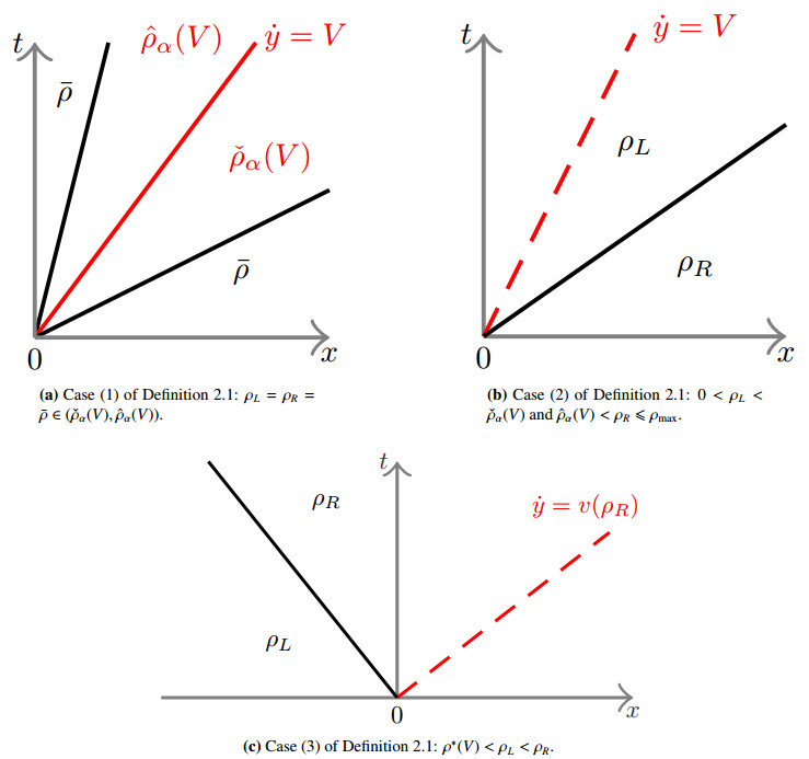
Definition 2.1. Let V∈[0,Vmax]. The constrained Riemann solver RV:[0,ρmax]2↦L1loc(IR;[0,ρmax]) for (2.1)-(2.3)-(2.4) and (2.9) is defined as follows:
1. If f(R(ρL,ρR)(V))>Fα(V)+VR(ρL,ρR)(V), then
| RV(ρL,ρR)(x/t)={R(ρL,ˆρα(V))(x/t)ifx<Vt,R(ˇρα(V),ρR)(x/t)ifx⩾Vt, |
andy(t)=Vt.
2. If VR(ρL,ρR)(V)⩽f(R(ρL,ρR)(V))⩽Fα(V)+VR(ρL,ρR)(V), then
| RV(ρL,ρR)=R(ρL,ρR)andy(t)=Vt. |
3. If f(R(ρL,ρR)(V))<VR(ρL,ρR)(V), then
| RV(ρL,ρR)=R(ρL,ρR)andy(t)=v(ρR)t. |
Note that when the constraint is enforced (1. in the above definition), a non-classical shock arises, which satisfies the Rankine-Hugoniot condition but violates the Lax entropy condition [17].
An illustration of each case in Definition 2.1 is shown in Figure 2. In particular, in Figure 2a, a non-classical shock (ˆρα,ˇρα) is shown.
In this section, we describe how to construct solutions to the coupled PDE-ODE system (2.5) adapting the wave front tracking method found in [6].
Let the initial density ρ0 and the initial trajectories of the autonomous vehicle (y0i)i∈{1,⋯,N} be known. Following [13], we can construct a density mesh Mn on the interval [0,ρmax] and a velocity mesh Vn on the interval [0,Vmax] such that (ˇρα(Vi),ˆρα(Vi))∈(Mn)2 for every i∈{1,⋯,N} and for every Vi∈Vn. We recall that Vi(t) is the speed of the ith autonomous vehicle at time t. Simultaneously, for every i∈{1,⋯,N}, we consider a sequence of piecewise constant functions (Vni)n∈IN and a sequence (ρn0)n∈IN having both a finite number of discontinuities such that
| limn→+∞‖ | (2.10) |
| (2.11) |
Remark 1. Hereafter, the term "approximately" means that a rarefaction wave is split into a fan of rarefaction shocks such that the left and the right densities of each rarefaction shock belongs to the state mesh .
Next, we describe the steps to construct the solution of the PDE-ODE system using the wave-front tracking method.
Step 1 For every AV , we solve approximately the constrained Riemann problem at as described in Section 2.2. This is done for with where is the first time when one of the AVs changes its speed.
Step 2 At each point of discontinuity of different from , we solve approximately the standard Riemann problem over .
Step 3 By piecing solutions together, we construct a solution and for every , is solution of
until two waves meet at .
Step 4 Now we check the value of :
If , then the approximate solution is still a piecewise constant function verifying for almost every . Thus, Step 1, Step 2 and Step 3 are repeated until two waves meet at a new , which is repeated until .
If , the constrained Riemann problem is solved over as previously replacing by for every where is the second time when one of the AVs changes its speed.
Using this approach, we construct an approximate solution of Eqs (2.1), (2.3) and (2.4).
In this section, we first present the Cauchy problem and prove existence of solutions. Next, building on this, we present and prove existence of solutions for the optimal control problem.
Let be the total variation and the set of functions of bounded variation endowed with the norm , (for more details, see [12]). Consider an initial density and initial positions of the AVs each of which has the following maximal speeds .
Definition 3.1. The -tuple provides a solution to Eqs (2.1), (2.3) and (2.4) if the following conditions hold.
1. .
2. For every , .
3. is a weak solution of , .
4. For every , for all and for every , it holds
| (3.1) |
5. For a.e. , for every ,
6. For a.e. , for every ,
Remark 2. Note that the Cauchy problem (2.1), (2.3) and (2.4) has previously been studied in [9,13,18,19] with only one autonomous vehicle ( in (2.3) and (2.4)). In the case where the maximum speed of the AV is constant in time, the existence and the stability of solutions for (2.1), (2.3) and (2.4) in the sense of Definition 3.1 has been proven in [9,18,19], while when the maximum speed of the AV depends on time, the existence of solutions for (2.1), (2.3) and (2.4) has been proven in [13]. Therefore, the focus of this article is to extend the theory to the case of .
Let and introduce the class of admissible maximal speed . The sequence if, for every and for every ,
with is solution of Eq (2.3). Note that the set depends on the initial density and the initial position of the autonomous vehicles . When , an autonomous vehicle can never catch up with the autonomous vehicle in front. Similarly, mathematically speaking, two non-classical shocks cannot interact.
Let us now prove the existence of solutions.
Theorem 3.2. Let , and let us assume that , and . Then, the Cauchy problem (2.1), (2.3) and (2.4) admits a solution in the sense of Definition 3.1.
Proof. Let us construct piecewise constant approximate solutions of (2.1), (2.3) and (2.4) using the wave-front tracking method described in Section 2.3. Then, let us introduce the following Glimm functional defined by
| (3.2) |
Roughly speaking, is a function created to compensate the possible interactions between the classical wave-fronts (shocks and rarefaction) and the autonomous vehicle. Moreover,
It is clear that is well-defined for a.e. and it changes only at discontinuity points of with or when two wave-fronts interacts (shocks, rarefaction and non-classical shocks). Hence, we have the following possibilities:
Let us assume that an interaction occurs at time at some distance from . In this case, either two shocks collide or a shock and a rarefaction interact. In both cases, we have and, for every , and leading to
Since , all possible interactions between classical waves (shocks and rarefaction) and the autonomous vehicle are described in [9,18]. In that case, for every , . From [18, Lemma 2], . Therefore, .
If , then we can refer to [13] when a jump occur in . In fact, from [13, Lemma 3.1,Lemma 3.2,Lemma 3.3], .
From this we conclude that
| (3.3) |
Then, from Eqs (2.10), (2.11) and (3.3), we get
| (3.4) |
Since and there exists such that , we can apply [13, Lemma 3.4]. Thus, up to a subsequence, we have
| (3.5a) |
| (3.5b) |
| (3.5c) |
with . In [13, Proof of Theorem 3.1], it is shown that the limit is a solution of (2.1), (2.3) and (2.4) in the sense of Definition 3.1. This can be applied in this context, since .
In this section we describe the optimal control problem and prove that it has at least one solution. We want to minimize the fuel consumption of the overall traffic flow by controlling the maximal speed of the AVs denoted by .
For this, we quantify the fuel consumption as a function of the vehicle density, which can be integrated over the entire roadway to calculate the total fuel consumed. Generally, fuel consumption increases with the speed of the vehicle, as shown by [1] and [2], with a nonlinear relationship between speed and fuel consumption. Using the fuel consumption rates of four different commercially available vehicles, [22] obtained the following best-fit model for fuel rate in liters per hour (/h) as a function of speed in kilometers per hour (km/h):
Using the relationship between speed and fuel rate (depicted in Figure 3a), as well as the relationship between density and speed in Eq (2.2) obtained by assuming the LWR model, it is possible to compute the fuel rate of the entire traffic flow, referred to as the bulk fuel rate as a function of traffic density with units /h/km by computing:
| (3.6) |
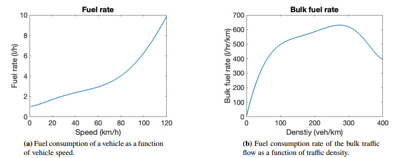
where is specified by the fundamental diagram (2.2). The resulting fuel-density relationship for the entire traffic flow is presented in Figure 3b.
The goal is to select the optimal AV trajectory to minimize the average fuel consumption of all vehicles in the bulk traffic flow. Therefore, we solve the following problem.
Problem. Let , , and such that . Fix and for every , . Find such that
| (3.7) |
where is the solution of (2.1), (2.3) and (2.4) associated to .
The functional represents the average fuel consumption computed on a highway section of length km between time 0 and . With this problem identified, we prove the main result:
Theorem 3.3. The optimal control problem Eq (3.7) has at least one optimal solution.
Proof. There exists a minimizing sequence verifying that
with and for every , .
Fix . Since and , there exists an approximate density of and an approximate maximum speed of such that
| (3.8) |
| (3.9) |
for every . As in the proof of Theorem 3.2, we construct an approximate solution of (2.1), (2.3) and (2.4) such that
| (3.10) |
Then, up to a subsequence, converges to a solution of (2.1), (2.3) and (2.4) with as and
| (3.11) |
In particular, we have
Moreover, using Eqs (3.10), (3.11) and , there exists a positive constant, still denoted by , independent of and such that
By the dominated convergence theorem,
| (3.12) |
Using that is a minimizing sequence and Eq (3.9), we deduce that, for every ,
| (3.13) |
and
| (3.14) |
From Eq (3.12), there exists a function strictly increasing such that
| (3.15) |
Using (3.13), we have
| (3.16) |
Note that is not a minimizing sequence. Helly's Theorem, see [24, Theorem 7.25], implies that there exists a function and a subsequence of , still denoted by , such that converges to in and for any . From Eq (3.16), we have
| (3.17) |
Note that is an approximate solution of (2.1), (2.3) and (2.4) with . As in the proof of Theorem 3.2, we have
| (3.18) |
Then, up to a subsequence, converges to a solution of Eqs (2.1), (2.3) and (2.4) with as and
| (3.19) |
In particular, we have
and for every
| (3.20) |
Moreover, using Eqs (3.18), (3.19) and , there exists a positive constant, still denoted by , independent of such that
By dominated convergence theorem,
| (3.21) |
where is a solution of Eqs (2.1), (2.3) and (2.4) with . Using that is a minimizing sequence, Eqs (3.15) and (3.21), we deduce that
| (3.22) |
From Eqs (3.20) and (3.14) with , for every , we have
| (3.23) |
Combining Eqs (3.17), (3.22) and (3.23), we conclude that is an optimal solution of Eq (3.7).
Lemma 3.4. The cost function is not differentiable with respect to .
Proof. To prove Lemma 3.4, it is enough to exhibit an example. Let , , and one autonomous vehicle drives on the road (), we assume that, for every , where is defined in Eq (2.6) and . Then the solution of Eqs (2.1), (2.3) and (2.4) associated to , and is, for every ,
| (3.24) |
Let and we denote by the solution of Eqs (2.1), (2.3) and (2.4) associated to , and . In this case, we have . Thus the flux constraint is active and so a non-classical shock is created. We deduce that, for every , for every ,
| (3.25) |
with and . Using Eqs (3.24) and (3.25), we conclude that the expression
| (3.26) |
does not define any -function.
Remark 3. Note that the optimal control problem (3.7) may admit multiple solutions. For instance, if the initial datum and , then is a constant function. Therefore, any such that is an optimal solution of (3.7).
In this section, we present numerical examples to demonstrate how AVs can be used as moving bottlenecks to control the flow of traffic and optimize the fuel consumption of not only the individual AVs, but also the entire traffic flow. First we present the numerical method to implement the control and then we introduce a numerical example to demonstrate the ability of AVs to act as moving bottlenecks for traffic control.
For a given initial traffic state (density distribution on the roadway) and starting position of the AVs, the optimal trajectory of each AV is computed such that it minimizes the total fuel consumption of the entire traffic flow. The optimal trajectory of each AV consists of a series of speeds to drive at for a corresponding time interval. This is based on the predicted traffic state and position of each AV as solved using the coupled ODE-PDE system.
Let be the number of time intervals and the number of autonomous vehicles. The AVs adjust their driving speed times during the experiment duration. We determine the speed profile for each AV by solving the following approximate optimization problem
| (4.1) |
where the cost function is defined in Eq (3.7) and, for every ,
| (4.2) |
with and .
The optimization problem (4.1) is solved using the genetic algorithm as implemented in the Matlab Global Optimization Toolbox (\texttt{ga()}) while the the solution of Eqs (2.1), (2.3) and (2.4) with as defined in Eq (4.2) is solved using the wave-front tracking algorithm described in Section 2.3.
Remark 4. Note that in our algorithm, in contrast to the theory, two autonomous vehicles are allowed to interact, leading to a possible interaction between two non-classical shocks since the constraint does not appear explicitly. However, this will not happen given that each optimal solution belongs to the class of admissible maximum speed , making it impossible for two AVs to reach each other and interact.
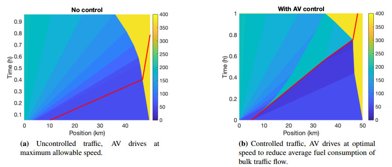
Using the implementation of the numerical method described in Section 4.1, numerical examples are conducted to demonstrate the control of AVs to act as a moving bottleneck and reduce the fuel consumption of the overall traffic flow. The numerical experiment is conducted over a stretch of highway ( km and km in Eq (3.7)) over the course of one hour ( hour in Eq (3.7)). The maximum speed of each AV on the roadway is km/h. The maximum (jam) density on the roadway is considered to be 400 veh/km. Each AV has influence over one of the two lanes ().
We consider two optimal control approaches for the AV: one in which each AV selects an optimal constant speed for the duration of the experiment, and another in which two AVs are allowed to select the optimal speed at up to six distinct points in the simulation.
We consider the initial traffic state
and allow the AV to change control speed up to to three times in the one hour experiment.
As seen in Figure 4, if the AV drives at the maximum possible velocity at all times, the AV encounters the leading edge of the shock wave after roughly 0.4 h. This results in an average fuel consumption of 3.87 per vehicle. However, when the AV is acting as a moving bottleneck to control the traffic and reduce the fuel consumption, it is able to achieve a lower density gap between the wave and the AV as seen in Figure 4b. By using the control strategy optimized with the genetic algorithm, the average fuel consumption for the same traffic flow is reduced to 3.72 per vehicle, a reduction of 3.7% on average across all vehicles.
In this work we study a coupled PDE-ODE framework to model the impact of multiple AVs being used as moving bottlenecks to control the flow of traffic and reduce the overall fuel consumption of the entire traffic stream. The main traffic flow is described by a scalar conservation law while the controlled vehicles are described via ODEs. The prove the existence of solutions for the coupled PDE-ODE systems and show how to compute analytically solutions to the Riemann problem and to the Cauchy problem via wave-front tracking approximations. We define an optimal control problem which consists in minimizing the total fuel consumption, using the autonomous vehicles speeds as control variables. We prove that the optimal control problem (3.7), admits at least one optimal solution. We solve numerically the optimal control problem (3.7) by using a genetic algorithm. For the numerical solution, the traffic flow and AVs as moving bottlenecks are simulated using wave-front tracking.
The first author is supported by the European Research Council (ERC) under the European Union's Horizon 2020 research and innovation programme (grant agreement No 694126-DYCON)
The authors declare there is no conflict of interest.
| [1] |
K. Ahn, H. Rakha, A. Trani, M. Van Aerde, Estimating vehicle fuel consumption and emissions based on instantaneous speed and acceleration levels, J Transp Eng, 128 (2002), 182–190. https://doi.org/10.1061/(ASCE)0733-947X(2002)128:2(182) doi: 10.1061/(ASCE)0733-947X(2002)128:2(182)

|
| [2] | I. M. Berry, The effects of driving style and vehicle performance on the real-world fuel consumption of US light-duty vehicles, Doctoral Thesis of Massachusetts Institute of Technology, Cambridge, 2010. |
| [3] |
C. Chalons, M. L. Delle Monache, P. Goatin, A conservative scheme for non-classical solutions to a strongly coupled pde-ode problem, Interfaces Free. Boundaries, 19 (2017), 553–570. https://doi.org/10.4171/IFB/392 doi: 10.4171/IFB/392
|
| [4] | M. Čičić, K. H. Johansson, Traffic regulation via individually controlled automated vehicles: a cell transmission model approach, 2018 21st International Conference on Intelligent Transportation Systems (ITSC), (2018), 766–771. |
| [5] | S. Cui, B. Seibold, R. Stern, D. B. Work, Stabilizing traffic flow via a single autonomous vehicle: Possibilities and limitations, Proceedings of the IEEE Intelligent Vehicles Symposium, (2017), 1336–1341. |
| [6] |
C. M. Dafermos, Polygonal approximations of solutions of the initial value problem for a conservation law, J. Math. Anal. Appl., 38 (1972), 33–41. https://doi.org/10.1016/0022-247X(72)90114-X doi: 10.1016/0022-247X(72)90114-X
|
| [7] |
L. Davis, Effect of adaptive cruise control systems on traffic flow, Phys Rev E, 69 (2004), 066110. https://doi.org/10.1103/PhysRevE.69.066110 doi: 10.1103/PhysRevE.69.066110
|
| [8] |
M. L. Delle Monache, P. Goatin, A front tracking method for a strongly coupled PDE-ODE system with moving density constraints in traffic flow, DISCRETE CONT DYN-S, 7 (2014), 435–447. https://doi.org/10.3934/dcdss.2014.7.435 doi: 10.3934/dcdss.2014.7.435
|
| [9] |
M. L. Delle Monache, P. Goatin, Scalar conservation laws with moving constraints arising in traffic flow modeling: an existence result, J Differ Equ, 257 (2014), 4015–4029. https://doi.org/10.1016/j.jde.2014.07.014 doi: 10.1016/j.jde.2014.07.014
|
| [10] |
M. L. Delle Monache, P. Goatin, Stability estimates for scalar conservation laws with moving flux constraints, Netw. Heterog. Media, 12 (2017), 245–258. https://doi.org/10.3934/nhm.2017010 doi: 10.3934/nhm.2017010
|
| [11] |
M. L. Delle Monache, T. Liard, B. Piccoli, R. Stern, D. Work, Traffic reconstruction using autonomous vehicles, SIAM J Appl Math, 79 (2019), 1748–1767. https://doi.org/10.1137/18M1217000 doi: 10.1137/18M1217000
|
| [12] | L. C. Evans, R. F. Gariepy, Measure Theory and Fine Properties of Functions, Boca Raton: CRC Press, 1991. |
| [13] |
M. Garavello, P. Goatin, T. Liard, B. Piccoli, A multiscale model for traffic regulation via autonomous vehicles, J Differ Equ, 269 (2020), 6088–6124. https://doi.org/10.1016/j.jde.2020.04.031 doi: 10.1016/j.jde.2020.04.031
|
| [14] | M. Guériau, R. Billot, N. E. El Faouzi, J. Monteil, F. Armetta, S. Hassas, How to assess the benefits of connected vehicles? A simulation framework for the design of cooperative traffic management strategies. Transp Res Part C Emerg Technol, 67 (2016), 266–279. https://doi.org/10.1016/j.trc.2016.01.020 |
| [15] | K. Huang, X. Di, Q. Du, X. Chen, Stabilizing traffic via autonomous vehicles: A continuum mean field game approach, 2019 IEEE Intelligent Transportation Systems Conference (ITSC), (2019), 3269–3274. |
| [16] |
F. Knorr, D. Baselt, M. Schreckenberg, M. Mauve, Reducing traffic jams via vanets, IEEE Transactions on Vehicular Technology, 61 (2012), 3490–3498. https://doi.org/10.1109/TVT.2012.2209690 doi: 10.1109/TVT.2012.2209690
|
| [17] |
P. D. Lax, Hyperbolic systems of conservation laws II, Commun. Pure Appl. Math., 10 (1957), 537–566. https://doi.org/10.1002/cpa.3160100406 doi: 10.1002/cpa.3160100406
|
| [18] |
T. Liard, B. Piccoli, On entropic solutions to conservation laws coupled with moving bottlenecks, Commun Math Sci, 19 (2021), 919–945. https://doi.org/10.4310/CMS.2021.v19.n4.a3 doi: 10.4310/CMS.2021.v19.n4.a3
|
| [19] |
T. Liard, B. Piccoli, Well-posedness for scalar conservation laws with moving flux constraints, SIAM J Appl Math, 79 (2019), 641–667. https://doi.org/10.1137/18M1172211 doi: 10.1137/18M1172211
|
| [20] |
M. J. Lighthill, G. B. Whitham, On kinematic waves II. A theory of traffic flow on long crowded roads, Proc. R. Soc. London A: Math. Phys. Sci., 229 (1955), 317–345. https://doi.org/10.1098/rspa.1955.0089 doi: 10.1098/rspa.1955.0089
|
| [21] |
G. Piacentini, P. Goatin, A. Ferrara, Traffic control via moving bottleneck of coordinated vehicles, IFAC-PapersOnLine, 51 (2018), 13–18. https://doi.org/10.1016/j.ifacol.2018.06.192 doi: 10.1016/j.ifacol.2018.06.192
|
| [22] | R. A. Ramadan, B. Seibold, Traffic flow control and fuel consumption reduction via moving bottlenecks, arXiv: 1702.07995, [Preprint], (2017) [cited 2023 April 07 ]. Available from: https://doi.org/10.48550/arXiv.1702.07995 |
| [23] | P. I. Richards, Shock waves on the highway, Oper. Res., 4 (1956), 42–51. https://doi.org/10.1287/opre.4.1.42 |
| [24] | W. Rudin, Principles of mathematical analysis, New York: McGraw-hill, 1976. |
| [25] | R. E. Stern, S. Cui, M. L. Delle Monache, R. Bhadani, M. Bunting, M. Churchill, et al., Dissipation of stop-and-go waves via control of autonomous vehicles: Field experiments, Transp Res Part C Emerg Technol, 89 (2018), 205–221. |
| [26] |
A. Talebpour, H. S. Mahmassani, Influence of connected and autonomous vehicles on traffic flow stability and throughput, Transp Res Part C Emerg Technol, 71 (2016), 143–163. https://doi.org/10.1007/s00115-018-0494-4 doi: 10.1007/s00115-018-0494-4
|
| [27] | E. Vinitsky, K. Parvate, A. Kreidieh, C. Wu, A. Bayen, Lagrangian control through deep-RL: Applications to bottleneck decongestion, 2018 21st International Conference on Intelligent Transportation Systems (ITSC), (2018), 759–765. https://doi.org/10.1016/j.trc.2016.07.007 |
| 1. | Zhexian Li, Michael W. Levin, Xu Qu, Raphael Stern, A Network Traffic Model for the Control of Autonomous Vehicles Acting as Moving Bottlenecks, 2023, 24, 1524-9050, 9004, 10.1109/TITS.2023.3271187 | |
| 2. | H. Wang, H. Nick Zinat Matin, M. L. Delle Monache, 2024, Reinforcement learning-based adaptive speed controllers in mixed autonomy condition, 978-3-9071-4410-7, 1869, 10.23919/ECC64448.2024.10590883 | |
| 3. | M. L. Delle Monache, C. Pasquale, M. Barreau, R. Stern, 2022, New frontiers of freeway traffic control and estimation, 978-1-6654-6761-2, 6910, 10.1109/CDC51059.2022.9993221 | |
| 4. | Han Wang, Zhe Fu, Jonathan W. Lee, Hossein Nick Zinat Matin, Arwa Alanqary, Daniel Urieli, Sharon Hornstein, Abdul Rahman Kreidieh, Raphael Chekroun, William Barbour, William A. Richardson, Dan Work, Benedetto Piccoli, Benjamin Seibold, Jonathan Sprinkle, Alexandre M. Bayen, Maria Laura Delle Monache, Hierarchical Speed Planner for Automated Vehicles: A Framework for Lagrangian Variable Speed Limit in Mixed-Autonomy Traffic, 2025, 45, 1066-033X, 111, 10.1109/MCS.2024.3499212 | |
| 5. | Kristina Maier, Martin Weiser, Tim Conrad, Hybrid PDE–ODE models for efficient simulation of infection spread in epidemiology, 2025, 481, 1364-5021, 10.1098/rspa.2024.0421 | |
| 6. | Chiara Daini, Maria Laura Delle Monache, Paola Goatin, Antonella Ferrara, Traffic Control via Fleets of Connected and Automated Vehicles, 2025, 26, 1524-9050, 1573, 10.1109/TITS.2024.3506703 |
Figures(4)
Thibault Liard, Raphael Stern, Maria Laura Delle Monache. A PDE-ODE model for traffic control with autonomous vehicles[J]. Networks and Heterogeneous Media, 2023, 18(3): 1190-1206. doi: 10.3934/nhm.2023051

 DownLoad:
