Iterative learning algorithms for boundary tracing problems of nonlinear fractional diffusion equations

1.   Introduction

In this paper, we consider boundary tracing problem of nonlinear fractional diffusion equations with Neumann boundary condition

by iterative learning algorithms, where $D_{t}^{\alpha}$ is the Caputo fractional derivative of order $\alpha$, $0 < \alpha < 1$, $(x, t)\in\Omega_{T}\triangleq [0, 1]\times [0, T]$ and $F(x, t, \varphi, \varphi_{x})$ is the nonlinear function.

The basic idea of iterative learning control (ILC) ^[1,4,16] can be traced back to Garden ^[8] in 1967 and Uchiyama ^[28] in 1978. ILC is a control method suitable for dealing with iterative systems, which uses information obtained from previous trial to improve the tracking performance of current trial. Owing to simplicity and effectiveness, ILC plays an important role in many fields and applications ^[9,10,14].

ILC schemes are widely used for ordinary differential equations (ODEs) ^{[23,25,26,29]}. However, there are few studies on its application to partial differential equations (PDEs) and fractional partial differential equations (FPDEs) ^[11,24]. Choi et al. ^[3] employed the characteristic line method and the Q-ILC method to study the ILC schemes of a first-order hyperbolic PDE system. Huang et al. ^[12] studied the $P$-type ILC scheme for boundary tracking of nonlinear hyperbolic parametric systems and evaluated the robustness of the scheme. Kang et al. ^[15] proposed a Newton-type ILC algorithm for nonlinear parametric equations and provided sufficient conditions for convergence of the Newton descent method using the $\lambda$-norm. Different from the convergence in the sense of the $\lambda$ norm, Dai et al. ^[5] derived the $P$-type ILC for linear parabolic parametric equations and proved its convergence in the sense of the $L^{2}$-norm and the $W^{1, 2}$-norm. Lan et al. ^[22] presented a second-order ILC method for a class of multi-agent systems (MAS) with time-delay distributed parameters and proved its convergence.

For the diffusion equation, Xu et al. ^[30] proposed $P$-type and $D$-type ILC methods for infinite-dimensional linear systems in Hilbert spaces. Huang et al. ^[13] extended ILC to solve the boundary tracking problem of inhomogeneous heat equations and provided evidence for the effectiveness of the $D$-type ILC scheme. Zhang et al. ^[32] presented a novel intermittent updating PD-type ILC algorithm for semi-linear distributed parameter systems with sensors or actuators, and provided convergence conditions for the output error. For the fractional diffusion equation, Lan et al. ^[20] discussed the $P$-type ILC of fractional order parameter exchange systems and demonstrated that the exchange system maintains traceability over two time periods. Lan et al. ^[21] proposed a second-order P-type ILC scheme for a class of linear fractional order distributed parameter systems and established a sufficient condition for convergence using $\lambda$-norm and generalized Gronwall inequality.

Overall, there have been relatively few studies on iterative learning control algorithms for fractional diffusion equations, which can describe a variety of memory materials and genetic processes ^[6,18]. Applying the ILC algorithm to fractional diffusion equations can improve control of the system for nonlocal transport phenomena and long-range memory effects, leading to faster convergence and improved tracking accuracy ^[19]. We aim to extend ILC to the nonlinear fractional diffusion equation and study their convergence. However, this work is challenging, as the difficulty lies in proving the convergence of the iterative learning control algorithm for fractional diffusion equations, with added challenges posed by the fractional derivatives and nonlinear source terms. Therefore, we assume that source term is Lipschitz continuous and employ Sobolev imbedding theorem to overcome difficulties in the proof.

In this paper, we consider boundary tracing problem of one dimensional fractional diffusion equation with input, state and output functions at the $k$-th iteration,

where $k$ denotes the iterative number of the process and $u^{k}, \varphi^{k}, y^{k}(t)$ are the input, state and output of the system at the $k$-th iteration respectively. The main idea is to adjust the control input $u^{k}(t)$ iteratively in order that system output {$y^{k}(t)$} can track the predefined target $y^{d}(t)$ when $k\rightarrow \infty$.

In addition, we make some assumptions about the functions in system (1.2). Suppose $c(t)$ and $d(t)$ are bounded and $F(x, t, \varphi^{k}, \varphi^{k}_{x})$ satisfies Lipschitz condition.

Assumption 1: The functions $c(t)$ and $d(t)$ satisfy

where $c_{1}, d_{1}, d_{2}$ are positive constants.

Assumption 2: The nonlinear function $F^{k}\triangleq F(x, t, \varphi^{k}, \varphi^{k}_{x})$ is Lipschitz continuous,

where $C_{F}$ is a constant.

This paper is organized as follows. Preliminaries are presented in Section 2. In Section 3, $P$-type ILC scheme, $PI^{\theta}$-type ILC scheme and corresponding convergence conditions are proposed for the nonlinear system. Numerical examples are given in Section 4 to illustrate the effectiveness of the methods. Finally, conclusions are drawn in Section 5.

2.   Preliminaries

To prepare for our subsequent analysis, it is essential to introduce some definitions, useful lemmas and theorems.

Definition 2.1. ^[17] Let $z(t)\in AC[0, T]$, the Caputo fractional derivative of order $\alpha$ is defined by

Definition 2.2. ^[17] Let $z(t)\in L(0, T)$, the Riemann-Liouville fractional integral of order $\alpha$ is defined by

Definition 2.3. ^[27] The two-parameter Mittag-Leffler function is defined by the series expansion

Lemma 2.1. ^[27] Suppose $0 < \alpha < 1$. Caputo fractional derivative and fractional integral of order $\alpha$ have the following relationship

Lemma 2.2. ^[7] Assume $x(t)$ be a differentiable function. The following relationship holds

Lemma 2.3. (Gronwall inequality ^[31]) Suppose a(t) is a nonnegative, nondecreasing, locally integrable function over $0\leq t_{0}\leq t\leq T$ and g(t) is a nonnegative, nondecreasing continuous function over $0\leq t_{0}\leq t\leq T$, $g(t)\leq M$, where $M$ is a postive constant. If u(t) is nonnegative and locally integrable function over $0\leq t_{0}\leq t\leq T$ and satisfies

then, we have

Theorem 2.1. (Sobolev imbedding theorem ^[2]) Let $\Omega \in R^{d}$ be a bounded Lipschitz domain and $1\leq p\leq\infty$. If $0\leq m < k-\frac{d}{p} < m+1$, the space $W^{k, p}(\Omega)$ is continuously imbedded in $C^{m, \alpha}(\overline{\Omega})$ for $\alpha = k-\frac{d}{p}-m$ and compactly imbedded in $C^{m, \beta}(\overline{\Omega})$ for all $0\leq \beta < \alpha$.

Remark 2.1. Using the Sobolbev imbedding theorem 2.1 in the case of d = 1, we can get

where $||\varphi(x, t)||^2_{H_{1}}\triangleq \int_{\Omega}^{}\varphi^{2}+\varphi^{2}_{x}dx$ and $C_{1}$ is a positive constant.

3.   ILC design for nonlinear systems

We need to give some necessary lemmas to obtain the convergence conditions for the ILC scheme.

Lemma 3.1. Suppose $e(t) \in AC[0, T)$ and $0.5 < \theta\leq 1$, then, we have

Proof. From the Definition 2.2 of fractional integral, we can get

where $|e|^2_{\lambda}\triangleq \mathop{\sup}\limits_{t\in[0, T]}\{e^{-\lambda t}|e(t)|^2, \lambda > 0\}$ and $|e(t)|$ represents absolute value of $e(t)$. Let $t-\tau = \omega$ and $\lambda \omega = v$, we have

From the definition of the Gamma function, we can get

This completes the proof.

Lemma 3.2. If $\psi$ satisfies the equation

we have

where

$|e(t)|$ represents absolute value of $e(t)$, $M = \mathop{\max}\limits_{t\in [0, T]}|D_{t}^{\alpha}\psi(0, t)|^{2}$, $c_{1} = \frac{\alpha^{\alpha}}{\alpha\Gamma(\alpha)e^{\alpha}}$, $\delta F = F(x, t, \varphi^{k+1}, \varphi_{x}^{k+1})-F(x, t, \varphi^{k}, \varphi_{x}^{k})$ and $\psi = \varphi^{k+1}-\varphi^{k}$.

Proof. (i) We firstly prove the formula (3.5). Multiplying both sides of the equation $D_{t}^{\alpha}\psi = \psi_{xx}+ \delta F$ by $\psi$ and integrating with respect to $x$, it yields

Based on Lemma 2.2, formula (1.3) and boundary condition, it is not hard to know

Using Young inequality (weighted form) and taking the positive constant $C_1$ in formula (2.1), it leads to

where $c_{2} = C_{F}^{2}+2C_{F}$. It follows from Theorem 2.1 that

Integrating both sides of the inequality with respect to $t$, by Lemma 2.1 we have

Using initial condition, we can get

Applying Lemma 2.3, we can obtain

Taking $\lambda$-norm on both sides of inequality, we can derive

(ii) We then prove the formula (3.6). Multiplying both sides of the equation $D_{t}^{\alpha}\psi = \psi_{xx}+\delta F$ by $\psi_{xx}$ and integrating with respect to $x$, it yields

By boundary condition, we get

Based on Lemma 2.2, it is not hard to know

We can conclude from the formula (1.3) that

Using Young inequality (weighted form), it leads to

where $M = \mathop{\max}\limits_{t\in [0, T]}|D_{t}^{\alpha}\psi(0, t)|^{2}$. Integrating both sides of the inequality about $t$ and using initial condition, according to Lemma 2.1 we get

Applying Lemma 2.3, we obtian

Taking $\lambda$-norm on both sides of inequality, we can derive

Since $t^{\alpha}e^{-\lambda t}$ gets the maximum value $\frac{\alpha^{\alpha}}{\lambda^{\alpha}e^{\alpha}}$ at $t = \frac{\alpha}{\lambda}$. Therefore, we can get

where $c_{1} = \frac{\alpha^{\alpha}}{\alpha\Gamma(\alpha)e^{\alpha}}$. Then, taking the maximum value on the left side of the inequality, we have

This completes the proof.

Lemma 3.3. If $\psi$ satisfies the equation

we have

where

$|e(t)|$ represents absolute value of $e(t)$, $M = \mathop{\max}\limits_{t\in [0, T]}|D_{t}^{\alpha}\psi(0, t)|^{2}$, $c_{1} = \frac{\alpha^{\alpha}}{\alpha\Gamma(\alpha)e^{\alpha}}$, $\delta F = F(x, t, \varphi^{k+1}, \varphi_{x}^{k+1})-F(x, t, \varphi^{k}, \varphi_{x}^{k})$, $\psi = \varphi^{k+1}-\varphi^{k}$ and $c_{3} = \frac{2\Gamma(2\theta-1)\gamma^{2}T}{\Gamma(\theta)^{2}}$.

Proof. (i) We firstly prove the formula (3.12). Multiplying both sides of the equation $D_{t}^{\alpha}\psi = \psi_{xx}+\delta F$ by $\psi$ and integrating with respect to $x$, it yields

Based on Lemma 2.2 and boundary condition, it is not hard to know

Using Young inequality (weighted form) and taking the positive constant $C_1$ in formula (2.1), we obtain

Applying Theorem2.1 and Lemma 3.1, it leads to

where $c_{3} = \frac{2\Gamma(2\theta-1)\gamma^{2}T}{\Gamma(\theta)^{2}}$. Integrating both sides of the inequality about $t$ and using initial condition, by Lemma 2.1 we get

It follows from Lemma 2.3 that

Taking $\lambda$-norm on both sides of inequality, we can derive

(ii) We then prove the formula (3.12). Multiplying both sides of the equation $D_{t}^{\alpha}\psi = \psi_{xx}+\delta F$ by $\psi_{xx}$ and integrating with respect to $x$, it yields

Based on boundary condition, it is not hard to know

According to Lemma 2.2, we obtain

Applying Lipschitz condition (1.3), we have

Using Young inequality (weighted form), it leads to

Integrating both sides of the inequality with respect to $t$ and using initial condition, by Lemma 2.1 and Lemma 3.1, we get

where $c_{3} = \frac{2\Gamma(2\theta-1)\gamma^{2}T}{\Gamma(\theta)^{2}}$. Using Lemma 2.3, we have

Taking $\lambda$-norm on both sides of inequality, similar to Lemma (3.2), we obtain

where $c_{1} = \frac{\alpha^{\alpha}}{\alpha\Gamma(\alpha)e^{\alpha}}$. This completes the proof.

3.1.   Open-loop $P$-type ILC

The open-loop P-type ILC scheme for Eq (1.2) is

where $e^{k}(t) = y^{d}(t)-y^{k}(t)$ denotes the output error and the learning gain $\beta$ is an unknown parameter to be determined later.

Theorem 3.1. For system (1.2) and the open-loop P-type law (3.13), if there exist a learning gain $\beta$ and a constant $l (l > 0)$ satisfying

where $\overline{\rho}_{1} = \mathop{\max}\limits_{t\in[0, T]}|1-\beta d(t)|$, then the output error $e^{k}$ can converge to the $\epsilon$-neighborhood of zero for any constant $\epsilon > 0$ in the sense of $\lambda$-norm as $k\rightarrow \infty$.

Proof. From the definition of error, we get

Based on the formula (3.13), it is not hard to know

Squaring both sides of the equation, we get

where $\overline{\rho}_{1} = \mathop{\max}\limits_{t\in[0, T]}|1-\beta d(t)|$ and $\overline{c} = \mathop{\max}\limits_{t\in [0, T]}|c(t)|$. Using Young inequality (weighted form) to ensure $(1+l)\overline{\rho}_{1}^{2}\leq 1$ and Theorem 2.1, we have

Taking $\lambda$-norm on both sides of inequality, we get

Using Lemma 3.2, we obtain

where

and $M_k = \mathop{\max}\limits_{t\in [0, T]}|D_{t}^{\alpha}\varphi^{k}(0, t)|^{2}$. Choosing $\lambda$ large enough so that $q_{1} < 1$, we get

where $\overline{\mu}_{1, k}\triangleq \mathop{\max}\limits_{m\in\{0, 1, \cdots, k\}}\mu_{1, m}$. We select $\lambda$ large enough so that $\overline{\mu}_{1, k}$ is sufficiently small. Therefore, to ensure $|e^{k+1}(t)|_{\lambda}^{2}\leq \epsilon^2$, it is sufficient to make

which means that the output error converges to the $\epsilon$-neighborhood of zero after finite step iteration ($k > \frac{2(\ln\epsilon-\ln|e^{0}|_{\lambda})}{\ln q_{1}}-1$).

Remark 3.1. Due to $q_{1}(\lambda)$ is a monotonic decreasing function of $\lambda$ and $(1+l)\overline{\rho}_{1}^{2} < 1$, we can see that the inequality $q_{1} < 1$ holds when $\lambda$ is large enough. From the definition of $\mu_{1, k}$, $\mu_{1, k}$ is proportional to $\lambda^{-\alpha}$. The number of iterations k is finited, so $\overline{\mu}_{1, k}$ is also proportional to $\lambda^{-\alpha}$ and $\overline{\mu}_{1, k}$ tends to zero when $\lambda$ is large enough.

Remark 3.2. In order to satisfy the convergence condition (3.14), the learning gain $\beta$ should satisfy

To ensure that the above inequality holds, parameter $l$ should satisfy

3.2.   Closed-loop $P$-type ILC

The closed-loop P-type ILC control scheme for (1.2) is

where $e^{k+1}(t) = y^{d}(t)-y^{k+1}(t)$ is the output error and the learning gain $\beta$ is an unknown parameter to be determined later.

Theorem 3.2. For system (1.2) and the ILC law (3.21), if there exist a learning gain $\beta$ and a constant $l (l > 0)$ satisfying

where $\overline{\rho}_{2} = \mathop{\max}\limits_{t\in[0, T]}\frac{1}{|1+\beta d(t)|}$, then the output error $e^{k}$ can converge to the $\epsilon$-neighborhood of zero for any constant $\epsilon > 0$ in the sense of $\lambda$-norm as $k\rightarrow \infty$.

Proof. From the definition of error, we get

Based on the formula ($3.21$), it is not hard to know

Simplifying the above equation, we have

Squaring both sides of the equation, we get

where $\overline{\rho}_{2} = \mathop{\max}\limits_{t\in[0, T]}\frac{1}{|1+\beta d(t)|}$ and $\overline{c} = \mathop{\max}\limits_{t\in [0, T]}|c(t)|$. Using Theorem 2.1 and Young inequality (weighted form) to ensure $(1+\overline{\rho}_{2}^{2}l)\overline{\rho}_{2}^{2} < 1$, we have

Taking $\lambda$-norm on both sides of inequality, we get

According to Lemma 3.2, we obtain

where

and $M_k = \mathop{\max}\limits_{t\in [0, T]}|D_{t}^{\alpha}\varphi^{k}(0, t)|^{2}$. Selecting a sufficiently large $\lambda$ such that $N_{1} < 1$, we can get

where $q_{2} = \frac{(1+\overline{\rho}_{2}^{2}l)\overline{\rho}_{2}^{2}}{1-N_{1}}$ and $\mu_{2, k} = \frac{N_{2, k}}{1-N_{1}}$. Using recursion, we get

where $\overline{\mu}_{2, k}\triangleq \mathop{\max}\limits_{m\in\{0, 1, \cdots, k\}}\mu_{2, m}$. We select $\lambda$ large enough such that $q_{2}$ is less than 1 and $\overline{\mu}_{2, k}$ is sufficiently small. Therefore, to ensure $|e^{k+1}(t)|_{\lambda}^{2}\leq \epsilon^2$, it is sufficient to make

which means that the output error converges to the $\epsilon$-neighborhood of zero after finite step iteration ($k > \frac{2(\ln\epsilon-\ln|e^{0}|_{\lambda})}{\ln q_{2}}-1$).

Remark 3.3. In order to satisfy the convergence condition (3.22), the learning gain $\beta$ should satisfy

3.3.   Open-loop $PI^{\theta}$-type ILC

The open-loop P-type ILC scheme for (1.2) is

where $e^{k}(t) = y^{d}(t)-y^{k}(t)$ denotes the output error and the learning gain $\beta$ and $\gamma$ are unknown parameters to be determined later.

Theorem 3.3. For system (1.2) and the ILC law (3.30), if the learning gain $\gamma$ is bounded, and there exist the learning gain $\beta$ and the constant $l (l > 0)$ satisfying

where $\overline{\rho}_{1} = \mathop{\max}\limits_{t\in[0, T]}|1-\beta d(t)|$, then the output error $e^{k}$ can converge to the $\epsilon$-neighborhood of zero for any constant $\epsilon > 0$ in the sense of $\lambda$-norm as $k\rightarrow \infty$.

Proof. By the definition of error, we have

Based on the formula (3.30), it is not hard to know

Applying Young inequality (weight form), we get

Using Theorem 2.1, it leads to

where $\overline{\rho}_{1} = \mathop{\max}\limits_{t\in[0, T]}|1-\beta d(t)|$ and $\overline{c} = \mathop{\max}\limits_{t\in [0, T]}|c(t)|$. Using Lemma 3.1, we obtain

where $c_{3} = \frac{2\Gamma(2\theta-1)\gamma^{2}T}{\Gamma(\theta)^{2}}$. Taking $\lambda$-norm on both sides of inequality, we have

According to Lemma 3.3, we get

where

and

Choosing $\lambda$ large enough such that $q_{3} < 1$, it leads to

where $\overline{\mu}_{3, k}\triangleq \mathop{\max}\limits_{m\in\{0, 1, \cdots, k\}}\mu_{3, m}$. We select $\lambda$ large enough such that $q_{3}$ is less than 1 and $\overline{\mu}_{3, k}$ is sufficiently small. Therefore, to ensure $|e^{k+1}(t)|_{\lambda}^{2}\leq \epsilon^2$, it is sufficient to make

which means that the output error converges to the $\epsilon$-neighborhood of zero after finite step iteration ($k > \frac{2(\ln\epsilon-\ln|e^{0}|_{\lambda})}{\ln q_{3}}-1$).

3.4.   Closed-loop $PI^{\theta}$-type ILC

The closed-loop P-type ILC scheme for (1.2) is

where $e^{k}(t) = y^{d}(t)-y^{k}(t)$ denotes the output error and the learning gain $\beta$ and $\gamma$ are unknown parameters to be determined later.

Theorem 3.4. For system (1.2) and the ILC law (3.36), if the learning gain $\gamma$ is bounded, and there exist the learning gain $\beta$ and the constant $l (l > 0)$ satisfying

where $\overline{\rho}_{2} = \mathop{\max}\limits_{t\in[0, T]}\frac{1}{|1+\beta d(t)|}$, then the output error $e^{k}$ can converge to the $\epsilon$-neighborhood of zero for any constant $\epsilon > 0$ in the sense of $\lambda$-norm as $k\rightarrow \infty$.

Proof. By the definition of error, we have

Based on the formula (3.36), it is not hard to know

Combining similar items, it leads to

Simplifying the above equation, we have

Applysing Young inequality (weighted form), we get

where $\overline{\rho}_{2} = \mathop{\max}\limits_{t\in[0, T]}\frac{1}{|1+\beta d(t)|}$ and $\overline{c} = \mathop{\max}\limits_{t\in [0, T]}|c(t)|$. Using Theorem 2.1, we obtain

According to Lemma 3.1, we have

where $c_{3} = \frac{2\Gamma(2\theta-1)\gamma^{2}T}{\Gamma(\theta)^{2}}$. Taking $\lambda$-norm on both sides of inequality, it leads to

Using Lemma 3.3, we can get

where

$C_{E} = 1+\frac{C_{F}^{2}E_{\alpha, 1}(C_{F}^{2}T^{\alpha})}{\lambda^{\alpha}}$ and $M_k = \mathop{\max}\limits_{t\in [0, T]}|D_{t}^{\alpha}\varphi^{k}(0, t)|^{2}$. Selecting a sufficiently large $\lambda$ such that $q_{4} < 1$, we can obtain

where $q_{4} = \frac{(1+\overline{\rho}_{2}^{2}l)\overline{\rho}_{2}^{2}}{1-N_{3}}$ and $\mu_{4, k} = \frac{N_{4, k}}{1-N_{3}}$. Using recursion, we get

where $\overline{\mu}_{4, k}\triangleq \mathop{\max}\limits_{m\in\{0, 1, \cdots, k\}}\mu_{4, m}$. We select $\lambda$ large enough such that $q_{4}$ is less than $1$ and $\overline{\mu}_{4, k}$ is sufficiently small. Therefore, to ensure $|e^{k+1}(t)|_{\lambda}^{2}\leq \epsilon^2$, it is sufficient to make

which means that the output error converges to the $\epsilon$-neighborhood of zero after finite step iteration ($k > \frac{2(\ln\epsilon-\ln|e^{0}|_{\lambda})}{\ln q_{4}}-1$).

4.   Numerical examples

In this section, we use the following numerical examples to verify convergence conditions of the open-loop $P$-type ILC, Closed-loop $P$-type ILC, open-loop $PI^{\theta}$-type ILC and Closed-loop $PI^{\theta}$-type ILC schemes. We can also observe the convergence speed of the four iterative learning algorithms from the numerical results.

Example 4.1. We consider a boundary tracing problem of one dimensional fractional diffusion equation

where

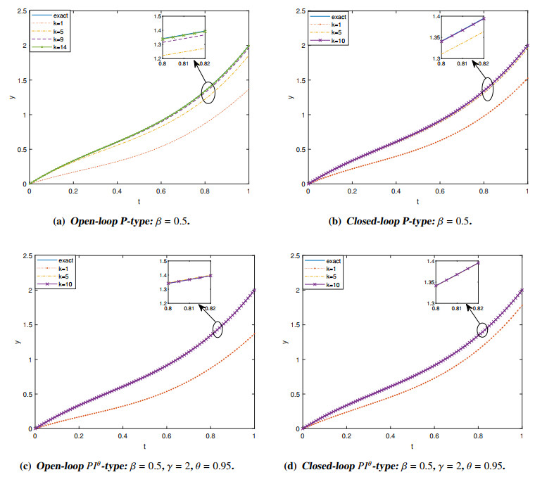
$\alpha = 0.9$ and $T = 1$. In this simulation, the output is determined as $y^{k}(t) = t\varphi^{k}(1, t)+(t^{2}-t+1)u^{k}(t)$, that is $c(t) = t$, $d(t) = (t^{2}-t+1)$. The output reference trajectory is $y^{d}(t) = 2(t^{3}-t^{2}+t)$.

Figure 1a displays the tracking performance of the open-loop $P$-type ILC, while Figure 1b shows the tracking performance of the closed-loop $P$-type ILC. Additionally, Figure 1c displays the tracking performance of the open-loop $PI^{\theta}$-type ILC, and Figure 1d shows the tracking performance of the closed-loop $PI^{\theta}$-type ILC.

Figure 2 displays the maximum norm of four ILC schemes at different iteration times, including the open-loop $P$-type, closed-loop $P$-type, open-loop $PI^{\theta}$-type, and closed-loop $PI^{\theta}$-type ILC schemes. The results demonstrate that the closed-loop-type ILC schemes converge faster than the open-loop-type ILC schemes.

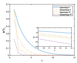
Figure 3a shows the unstable behavior of the open-loop ILC scheme. When $\beta$ is set to 2, the open-loop $P$-type ILC scheme fails to meet the convergence conditions. Figure 3b displays that the closed-loop $P$-type ILC scheme satisfies the convergence conditions and achieves faster convergence speed.

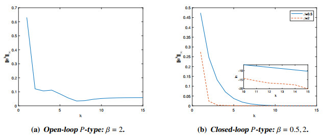
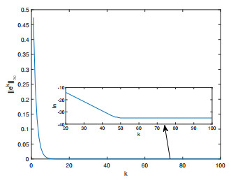
Figure 4 illustrates the convergence behavior of the maximum error $||e^{k}||_{\infty}$ of the closed-loop $P$-type ILC scheme over 100 iterations. Although the maximum error does not decrease at iteration $k = 50$, the scheme remains stable and does not diverge.

Tables 1 and 2 respectively provide the maximum error of open-loop $PI^{\theta}$-type and closed-loop $PI^{\theta}$-type schemes. Comparing the data of $PI^{\theta}$-type and $P$-type schemes in the tables, it can be observed that the $PI^{\theta}$-type ILC scheme converges faster than the $P$-type ILC scheme. Comparing the data of the $PI^{\theta}$-type $(0.5 < \theta < 1)$ and the $PI$-type $(\theta = 1)$ schemes in the tables, it can be observed that the $PI^{\theta}$-type ILC scheme converges faster than the $PI$-type ILC scheme.

5.   Conclusions

In this paper, we investigate iterative learning algorithms for boundary tracking of nonlinear fractional diffusion equation. We provide convergence conditions for open-loop $P$-type, closed-loop $P$-type, open-loop $PI^{\theta}$-type and closed-loop $PI^{\theta}$-type ILC algorithms. Numerical results demonstrate the effectiveness and stability of our proposed ILC schemes. Specifically, the closed-loop ILC schemes converge faster than the open-loop ILC schemes, and the $PI^{\theta}$-type ILC scheme outperforms the $P$-type and $PI$-type ILC schemes.

Acknowledgments

This research was supported by National Natural Science Foundation of China (No.11971387) and the fund of Sichuan Gas Turbine Establishment Aero Engine Corporation of China (GJCZ-2020-0018).

Conflict of interest

The authors declare that there is no conflict of interest.