


Figure 1.
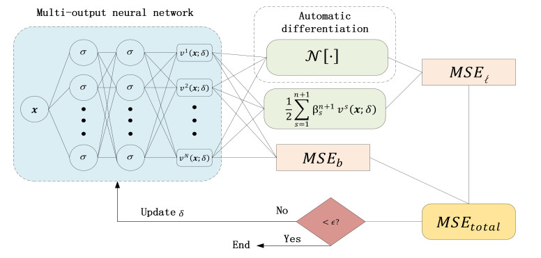
A multi-output neural network framework to solve nonlinear time distributed-order models, where MSE∗ represents the loss function.
In this article, a physics-informed neural network based on the time difference method is developed to solve one-dimensional (1D) and two-dimensional (2D) nonlinear time distributed-order models. The FBN-θ, which is constructed by combining the fractional second order backward difference formula (BDF2) with the fractional Newton-Gregory formula, where a second-order composite numerical integral formula is used to approximate the distributed-order derivative, and the time direction at time tn+12 is approximated by making use of the Crank-Nicolson scheme. Selecting the hyperbolic tangent function as the activation function, we construct a multi-output neural network to obtain the numerical solution, which is constrained by the time discrete formula and boundary conditions. Automatic differentiation technology is developed to calculate the spatial partial derivatives. Numerical results are provided to confirm the effectiveness and feasibility of the proposed method and illustrate that compared with the single output neural network, using the multi-output neural network can effectively improve the accuracy of the predicted solution and save a lot of computing time.
Citation: Wenkai Liu, Yang Liu, Hong Li, Yining Yang. Multi-output physics-informed neural network for one- and two-dimensional nonlinear time distributed-order models[J]. Networks and Heterogeneous Media, 2023, 18(4): 1899-1918. doi: 10.3934/nhm.2023080
| [1] | Qing Li, Steinar Evje . Learning the nonlinear flux function of a hidden scalar conservation law from data. Networks and Heterogeneous Media, 2023, 18(1): 48-79. doi: 10.3934/nhm.2023003 |
| [2] | Huanhuan Li, Meiling Ding, Xianbing Luo, Shuwen Xiang . Convergence analysis of finite element approximations for a nonlinear second order hyperbolic optimal control problems. Networks and Heterogeneous Media, 2024, 19(2): 842-866. doi: 10.3934/nhm.2024038 |
| [3] | Didier Georges . Infinite-dimensional nonlinear predictive control design for open-channel hydraulic systems. Networks and Heterogeneous Media, 2009, 4(2): 267-285. doi: 10.3934/nhm.2009.4.267 |
| [4] | Junjie Wang, Yaping Zhang, Liangliang Zhai . Structure-preserving scheme for one dimension and two dimension fractional KGS equations. Networks and Heterogeneous Media, 2023, 18(1): 463-493. doi: 10.3934/nhm.2023019 |
| [5] | Yaxin Hou, Cao Wen, Yang Liu, Hong Li . A two-grid ADI finite element approximation for a nonlinear distributed-order fractional sub-diffusion equation. Networks and Heterogeneous Media, 2023, 18(2): 855-876. doi: 10.3934/nhm.2023037 |
| [6] | Yinlin Ye, Hongtao Fan, Yajing Li, Ao Huang, Weiheng He . An artificial neural network approach for a class of time-fractional diffusion and diffusion-wave equations. Networks and Heterogeneous Media, 2023, 18(3): 1083-1104. doi: 10.3934/nhm.2023047 |
| [7] | Panpan Xu, Yongbin Ge, Lin Zhang . High-order finite difference approximation of the Keller-Segel model with additional self- and cross-diffusion terms and a logistic source. Networks and Heterogeneous Media, 2023, 18(4): 1471-1492. doi: 10.3934/nhm.2023065 |
| [8] | Martin Gugat, Alexander Keimer, Günter Leugering, Zhiqiang Wang . Analysis of a system of nonlocal conservation laws for multi-commodity flow on networks. Networks and Heterogeneous Media, 2015, 10(4): 749-785. doi: 10.3934/nhm.2015.10.749 |
| [9] | Jungang Wang, Qingyang Si, Jun Bao, Qian Wang . Iterative learning algorithms for boundary tracing problems of nonlinear fractional diffusion equations. Networks and Heterogeneous Media, 2023, 18(3): 1355-1377. doi: 10.3934/nhm.2023059 |
| [10] | Caterina Balzotti, Maya Briani, Benedetto Piccoli . Emissions minimization on road networks via Generic Second Order Models. Networks and Heterogeneous Media, 2023, 18(2): 694-722. doi: 10.3934/nhm.2023030 |
In this article, a physics-informed neural network based on the time difference method is developed to solve one-dimensional (1D) and two-dimensional (2D) nonlinear time distributed-order models. The FBN-θ, which is constructed by combining the fractional second order backward difference formula (BDF2) with the fractional Newton-Gregory formula, where a second-order composite numerical integral formula is used to approximate the distributed-order derivative, and the time direction at time tn+12 is approximated by making use of the Crank-Nicolson scheme. Selecting the hyperbolic tangent function as the activation function, we construct a multi-output neural network to obtain the numerical solution, which is constrained by the time discrete formula and boundary conditions. Automatic differentiation technology is developed to calculate the spatial partial derivatives. Numerical results are provided to confirm the effectiveness and feasibility of the proposed method and illustrate that compared with the single output neural network, using the multi-output neural network can effectively improve the accuracy of the predicted solution and save a lot of computing time.
With the continuous development and progress of computing technology over the past decade, deep learning has taken a big step on the road of evolution. Deep learning can be found in many fields, such as imaging and natural language. Scholars have begun to apply deep learning to solve some complex partial differential equations (PDEs), which include PDEs with high order derivatives [1], high-dimensional PDEs [2,3], subdiffusion problems with noisy data [4] and so on. Based on the deep learning method, Raissi et al. [5] proposed a novel algorithm called the physics informed neural network (PINN), which has made excellent achievements for solving forward and inverse PDEs. It integrates physical information described by PDEs into a neural network. In recent years, the PINNs algorithm has attracted extensive attention. To solve forward and inverse problems of integro-differential equations (IDEs), Yuan et al. [6] proposed auxiliary physics informed neural network (A-PINN). Lin and Chen [7] designed a two-stage physics informed neural network for approximating localized wave solutions, which introduces the measurement of conserved quantities in stage two. Yang et al. [8] developed Bayesian physics informed neural networks (B-PINNs) that takes Bayesian neural network and Hamiltonian Monte Carlo or the variational inference as a priori and posteriori estimators, respectively. Scholars have also presented other variant algorithms of PINN, such as RPINNs [9] and hp-VPINNs [10]. PINN has also achieved good performance for solving physical problems, including high-speed flows [11] and heat transfer problems [12]. In addition to integer-order differential equations, authors have studied the application of PINN in solving fractional differential equations such as fractional advection-diffusion equations (see Pang et al. [13] for fractional physics informed neural network (fPINNs)), high dimensional fractional PDEs (see Guo et al. [14] for Monte Carlo physics-informed neural networks (MC-PINNs)) and fractional water wave models (see Liu et al. [15] for time difference PINN).
In recent decades, fractional differential equations (FDEs) have been concerned and studied in many fields, such as image denoising [16] and physics [17,18,19]. The reason why fractional differential equations have attracted wide attention is that they can more clearly describe complex physical phenomena. As an indispensable part of fractional problems, distributed-order differential equations are difficult to solve due to the complexity of distributed-order operators. To solve the time multi-term and distributed-order fractional sub-diffusion equations, Gao et al. [20] proposed a second order numerical difference formula. Jian et al. [21] derived a fast second-order implicit difference scheme of time distributed-order and Riesz space fractional diffusion-wave equations and analyzed the unconditional stability and second-order convergence. Li et al. [22] applied the mid-point quadrature rule with finite volume method to approximate the distributed-order equation. For the nonlinear distributed-order sub-diffusion model [23], the distributed-order derivative and the spatial direction were approximated by the FBN-θ formula with a second-order composite numerical integral formula and the H1-Galerkin mixed finite element method, respectively. In [24], Guo et al. adopted the Legendre-Galerkin spectral method for solving 2D distributed-order space-time reaction-diffusion equations. For the two-dimensional Riesz space distributed-order equation, Zhang et al. [25] used Gauss quadrature to calculate the distributed-order derivative and applied an alternating direction implicit (ADI) Galerkin-Legendre spectral scheme to approximate the spatial direction. For the distributed-order fourth-order sub-diffusion equation, Ran and Zhang [26] developed new compact difference schemes and proved their stability and convergence. In [27,28], authors developed spectral methods for the distributed-order time fractional fourth-order PDEs.
As we know, distributed-order fractional PDEs can be regarded as the limiting case of multi-term fractional PDEs [29]. Moreover, Diethelm and Ford [30] have observed that small changes in the order of a fractional PDE lead to only slight changes in the final solution, which gives initial support to the employed numerical integration method. In view of this, we develop the FBN-θ [31,32] with a second-order composite numerical integral formula combined with a multi-output neural network for solving 1D and 2D nonlinear time distributed-order models. Based on the idea of using a single output neural network combined with the discrete scheme of fractional models [13], we also use a single output neural network combined with a time discrete scheme to solve the nonlinear time distributed-order models. However, the accuracy of the prediction solution calculated by the single output neural network scheme is low and the training progress takes a lot of time. Therefore, we introduce a multi-output neural network to obtain the numerical solution of the time discrete scheme. Compared with the single output neural network scheme, the proposed multi-output neural network scheme has two main advantages as follows:
● Saving more computing time. The multi-output neural network scheme makes the sampling domain of the collocation points from the spatiotemporal domain to the spatial domain, which decreases the number of the training dataset and thus reduces the training time.
● Improving the accuracy of predicted solution. Due to the discrete scheme of the distributed-order derivative, the n-th output item of the multi-output neural network will be constrained by the previous n−1 output items.
The remainder of this article is as follows: In Section 2, we show what the components of neural network are and how to construct a neural network. In Section 3, we give the lemmas used to approximate the distributed-order derivative and the process of building the loss function. In Section 4, we provide some numerical results to confirm the capability of our proposed method. Finally, we make some conclusions in Section 5.
In face of different objectives in various fields, scholars have developed many different types of neural networks, such as feed-forward neural network (FNN) [6], recurrent neural network (RNN) [33] and convolutional neural network (CNN) [34]. The FNN considered in this article can effectively solve most PDEs. Input layer, hidden layer and output layer are three indispensable components of FNN, which can be given, respectively, by
| input layer:Φ0(x)=x∈Rdin,hidden layers:Φk(x)=σ(WkΦk−1(x)+bk)∈Rλk,1≤k≤K−1,output layer:ΦK(x)=WKΦK−1(x)+bK∈Rdout. |
Wk∈Rλk×λk−1 and bk∈Rλk represent the weight matrix and the bias vector in the kth layer, respectively. We define δ={Wk,bk}1≤k≤K, which is the trainable parameters of FNN. λk represents the number of neurons included in the kth layer. σ is a nonlinear activation function. In this article, the hyperbolic tangent function [3,6] is selected as the activation function. There are many other functions that can be considered as activation functions, such as the rectified linear unit (ReLU) σ(x)=max{x,0} [4] and the logistic sigmoid σ(x)=11+e−x [35].
In this article, we consider a nonlinear distributed-order model with the following general form:
| {Dwtu+N(u)=f(x,t),(x,t)∈Ω×J,u(x,0)=u0(x),x∈ˉΩ, | (3.1) |
where Ω⊂Rd(d≤2) and J=(0,T]. N[⋅] is a nonlinear differential operator. Dwtu represents the distributed-order derivative and has the following definition:
| Dwtu(x,t)=∫10ω(α)C0Dαtu(x,t)dα, | (3.2) |
where ω(α)≥0, ∫10ω(α)dα=c0>0 and C0Dαtu(x,t) is the Caputo fractional derivative expressed by
| C0Dαtu(x,t)={1Γ(1−α)∫t0uη(x,η)(t−η)−αdη,0<α<1,ut(x,t),α=1. | (3.3) |
The specific boundary condition is determined by the practical problem.
For simplicity, choosing a mesh size Δα=12I, we denote the nodes on the interval [0,1] with coordinates αi=iΔα for i=0,1,2,⋯,2I. The time interval [0,T] is divided as the uniform mesh with the grid points tn=nΔt(n=0,1,2,⋯,N) and Δt=T/N is the time step size. We denote vn≈un=u(x,tn), un+12t=un+1−unΔt+O(Δt2) and un+12:=un+1+un2. vn is defined as the approximation solution of the time discrete scheme. The following lemmas are introduced to construct the numerical discrete formula of (3.1):
Lemma 3.1. (See [23]) Supposing ω(α)∈C2[0,1], we can get
| ∫10ω(α)dα=Δα2I∑k=0ciω(αi)−Δα212ω(2)(γ),γ∈(0,1), | (3.4) |
where
| ci={12,i=0,2I,1,otherwise. | (3.5) |
Lemma 3.2. From [23,31,32], the discrete formula of the Caputo fractional derivative (3.3) can be obtained by
| C0Dαtu(x,tn+12)=C0Dαtun+1+C0Dαtun2+O(Δt2)=Δt−αn+1∑s=0˜κ(α)n+1−sus+O(Δt2), | (3.6) |
where
| ˜κ(α)n+1−s={κ(α)02,s=n+1,κ(α)n−s+κ(α)n+1−s2,otherwise. | (3.7) |
The parameters κ(α)i(i=0,1,⋯,n+1) that are the coefficients of FBN-θ (θ∈[−12,1]) can be given by
| κ(α)i={2−α(1+αθ)(3−2θ)α,i=0,ϕ0κ(α)0ψ0,i=1,12ψ0[(ϕ0−ψ1)κ(α)1+ϕ1κ(α)0],i=2,1iψ03∑j=1[ϕj−1−(i−j)ψj]κ(α)i−j,i≥3, | (3.8) |
where
| ϕi={2α(θ−1)(αθ+1)+αθ(θ−32),i=0,−α(2θ2−3αθ+4αθ2−1),i=1,−αθ(12−θ+α−2αθ),i=2, | (3.9) |
and
| ψi={12(3−2θ)(1+αθ),i=0,−αθ2(3−2θ)−2(1−θ)(αθ+1),i=1,−12(2θ−1)(αθ+1)−2αθ(θ−1),i=2,−12αθ(1−2θ). | (3.10) |
Lemma 3.3. (See [23]) The distributed-order term Dωtu at t=tn+12 can be calculated by the following formula:
| Dωtu(x,tn+12)=Dωtun+1+Dωtun2+O(Δt2)=12n+1∑s=0βn+1sus+O(Δt2+Δα2), | (3.11) |
where
| βn+1s={ˆκn−s+ˆκn+1−s,0≤s<n+1,ˆκ0,s=n+1, | (3.12) |
and
| ˆκn−s=2I∑i=0φiΔtαiκ(αi)n−s,φi=Δαω(αi)ci. | (3.13) |
Based on the above lemmas, the discrete scheme of the distributed-order model (3.1) at t=tn+12(n=0,1,2,⋯,N−1) can be expressed by the following equality:
| 12n+1∑s=0βn+1svs+N(vn+12)=fn+12. | (3.14) |
Then we can obtain the system of equations as follows:
| {121∑s=0β1svs+N(v12)=f12,122∑s=0β2svs+N(v1+12)=f1+12,⋮12N∑s=0βNsvs+N(vN−12)=fN−12. | (3.15) |
The system of Eq (3.15) can be rewritten as the following matrix form:
| v(x)M+N(v(x))+v0(x)ρ0=f(x), | (3.16) |
where the symbols ρ0, v(x), f(x) and N(v(x)) are vectors, which are given, respectively, by
| ρ0=[12β10,12β20,12β30,⋯,12βN0],v(x)=[v1(x),v2(x),⋯,vN(x)],f(x)=[f12(x),f1+12(x),⋯,fN−12(x)],N(v(x))=[N(v12(x)),N(v1+12(x)),⋯,N(vN−12(x))]. |
The symbol M is an N×N matrix that has the following definition:
| M=(12β1112β21⋯12βN1012β22⋯12βN2⋮⋮⋮00⋯12βNN). |
Now, we introduce a multi-output neural network v(x;δ)=[v1(x;δ),v2(x;δ),⋯,vN(x;δ)] into Eq (3.16), which takes x as an input and is used to approximate time discrete solutions v(x)=[v1(x),v2(x),⋯,vN(x)]. This will result in a multi-output PINN ℓ(x)=[ℓ1(x),ℓ2(x),⋯,ℓN(x)]:
| ℓ(x)=v(x;δ)M+N(v(x;δ))+v0(x)ρ0−f(x), | (3.17) |
where ℓn+1(x) is denoted as residual error of the discrete scheme (3.14), which is given by
| ℓn+1(x)=12n+1∑s=1βn+1svs(x;δ)+N(vn+12(x;δ))+12βn+10v0(x)−fn+12(x),n=0,1,2,⋯,N−1. | (3.18) |
The loss function is constructed in the form of mean square error. Combined with the boundary condition loss, the total loss function can be expressed by the following formula:
| MSEtotal=MSEℓ+MSEb, | (3.19) |
where
| MSEℓ=1N×NxN∑j=1Nx∑i=1|ℓj(xiℓ)|2, | (3.20) |
and boundary condition loss
| MSEb=1N×NbN∑j=1Nb∑i=1|vj(xib;δ)−uj(xib)|2. | (3.21) |
Here, {xiℓ}Nxi=1 corresponds to the collocation points on the space domain Ω and {xib}Nbi=1 denotes the boundary training data. The schematic diagram of using the multi-output neural network scheme to solve nonlinear time distributed-order models is shown in Figure 1.
In this section, we consider two nonlinear time distributed-order equations to verify the feasibility and effectiveness of our proposed method. The performance is evaluated by calculating the relative L2 error between the predicted and exact solutions. The definition of relative L2 error is given by
| ||u−v||L2=√∑Nj=1∑Nxi=1|uj(xi)−vj(xi)|2√∑Nj=1∑Nxi=1|uj(xi)|2. | (4.1) |
Table 1 indicates which optimizer is selected for each example to minimize the loss function.
| Example | Optimizer | Learning rate | Iterations |
| 1 | Adam + L-BFGS | 0.001 | 20000 |
| 2 | Adam + L-BFGS | 0.001 | 20000 |
| 3 | Adam + L-BFGS | 0.001 | 20000 |
| 4 | L-BFGS | - | - |
 DownLoad:
CSV
DownLoad:
CSV
We use Python to code our algorithms and all codes run on a Lenovo laptop with AMD R7-6800H CPU @ 3.20 GHz and 16.0GB RAM.
Here, we solve the following distributed-order sub-diffusion model:
| ut+Dωtu−Δu−Δut+G(u)=f(x,t),(x,t)∈Ω×J, | (4.2) |
with boundary condition
| u(x,t)=0,x∈∂Ω,t∈ˉJ, | (4.3) |
and initial condition
| u(x,0)=u0(x),x∈ˉΩ, | (4.4) |
where the nonlinear term G(u)=u2. The symbol Δ is the Laplace operator. Based on Eqs (3.14)–(3.21), the loss function MSEtotal can be obtained by
| MSEtotal=MSEℓ+MSEb, |
where
| MSEℓ=1N×NxN∑j=1Nx∑i=1|ℓj(xiℓ)|2,MSEb=1N×NbN∑j=1Nb∑i=1|vj(xib;δ)−0|2. |
Example 1.
For this example, we set space domain Ω=(0,1) and time interval J=(0,12]. The training set consists of the boundary points and Nx=200 collocation points randomly selected in the space domain Ω. Choosing ω(α)=Γ(3−α) and the source term
| f(x,t)=2tsin(2πx)+Γ(3)t(t−1)lntsin(2πx)+4t2π2sin(2πx)+8tπ2sin(2πx)+(t2sin(2πx))2, |
then we can obtain the exact solution u(x,t)=t2sin(2πx).
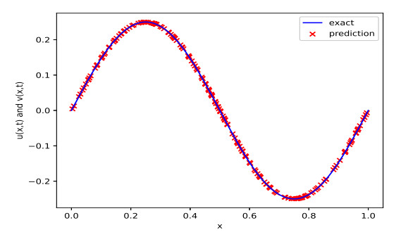
To evaluate the performance of our proposed method, the exact solution and the predicted solution solved by a multi-output neural network that consists of 6 hidden layers with 40 neurons in each hidden layer are showed in Figure 2.
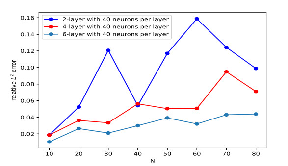
The influence of different network structures on our proposed method to solve Example 1 is presented in Table 2. The accuracy of the predicted solution fluctuates with different network architectures, and shows a fluctuating growth with the increase of the number of hidden layers. Based on the three network architectures, Figure 3 shows the behavior performance of the proposed method with gradual decrease of the time step size. With the increase of the number of grid points in the time interval, we observe that the behavior of relative L2 error generally presents an upward trend for fixed network architecture and expanding the depth of the hidden layer can effectively improve the accuracy of the predicted solution.
 |
20 | 30 | 40 | 50 | 60 |
| 2 | 3.583482e-02 | 7.850782e-02 | 5.238403e-02 | 1.143600e-01 | 3.761048e-02 |
| 4 | 3.815002e-02 | 5.144618e-02 | 3.622479e-02 | 2.317038e-02 | 3.721057e-02 |
| 6 | 2.433509e-02 | 1.216386e-01 | 2.638224e-02 | 2.837553e-02 | 2.682958e-02 |
DownLoad:
CSV
Numerical results calculated by the single output neural network and multi-output neural network schemes are presented in Table 3, where we select 200 collocation points in the given spatial domain by random sampling method and set N=10, θ=1 and Δα=1500. It is easy to find that the accuracy of the predicted solution calculated by the multi-output neural network scheme is higher than that solved by the single output neural network scheme and replacing single output neural network with multi-output neural network can save a lot of computing time.
| Neural network | Layers | Neurons | Relative L2 error | CPU time (s) |
| multi-output | 4 | 20 | 1.948281e-02 | 32.80 |
| 40 | 1.858120e-02 | 44.45 | ||
| 6 | 20 | 9.724722e-03 | 51.40 | |
| 40 | 1.024869e-02 | 65.88 | ||
| single output | 4 | 20 | 8.741336e-02 | 661.99 |
| 40 | 2.702814e-02 | 742.17 | ||
| 6 | 20 | 2.937448e-02 | 748.31 | |
| 40 | 2.278774e-02 | 840.09 |
DownLoad:
CSV
Example 2.
In this numerical example, considering the space domain Ω=(0,1)×(0,1), the time interval J=(0,12], ω(α)=Γ(3−α) and the exact solution u(x,y,t)=t2sin(2πx)sin(2πy), the source term can be given by
| f(x,y,t)=2tsin(2πx)sin(2πy)+Γ(3)t(t−1)lntsin(2πx)sin(2πy)+8t2π2sin(2πx)sin(2πy)+16tπ2sin(2πx)sin(2πy)+(t2sin(2πx)sin(2πy))2. |
The training dataset is shown in Figure 5 and the collocation and boundary points are selected by random sampling method.
To better illustrate the behavior of the predicted solution, Figure 4 portrays the contour plot of the exact and predicted solutions, where the training set consists of 961 collocation points and 124 boundary points selected by the equidistant uniform sampling method and the network architecture consists of 12 hidden layers with 60 neurons per layer.
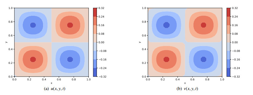
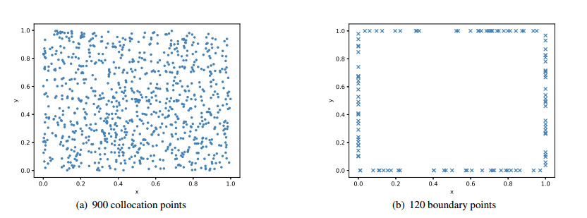
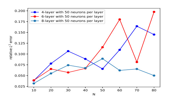
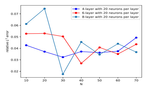
Table 4 shows the impact of depth and width of the network on the accuracy of the predicted solution. In Figure 6, we present the behavior of how relative L2 error changes with respect to different grid points N. Combined with Table 4 and Figure 6, we observe that increasing the number of hidden layers or neurons has a positive effect on reducing relative L2 error in general.
 |
20 | 30 | 40 | 50 | 60 |
| 4 | 1.155984e-01 | 1.101123e-01 | 7.228454e-02 | 7.787707e-02 | 4.492646e-02 |
| 6 | 6.273340e-02 | 6.088659e-02 | 9.802474e-02 | 6.536637e-02 | 6.245142e-02 |
| 8 | 6.163051e-02 | 7.424834e-02 | 6.844676e-02 | 5.500003e-02 | 5.169303e-02 |
DownLoad:
CSV
The results shown in Table 5 reveal the performance of the single output neural network and multi-output neural network schemes, where we select 40 boundary points and 200 collocation points in the given spatial domain by random sampling method and set N=10, θ=1 and Δα=1500. One can see that using multi-output neural network effectively improves the precision and reduces the computing time.
| Neural network | Layers | Neurons | Relative L2 error | CPU time (s) |
| multi-output | 4 | 20 | 1.080369e-01 | 52.84 |
| 40 | 7.472573e-02 | 66.05 | ||
| 6 | 20 | 6.654115e-02 | 72.71 | |
| 40 | 7.937601e-02 | 93.77 | ||
| single output | 4 | 20 | 3.443264e-01 | 731.22 |
| 40 | 7.054495e-01 | 728.11 | ||
| 6 | 20 | 2.636401e-01 | 772.08 | |
| 40 | 1.410780e-01 | 892.94 |
DownLoad:
CSV
Further, we consider the following distributed-order fourth-order sub-diffusion model:
| ut+Dωtu−Δu+Δ2u+G(u)=f(x,t),(x,t)∈Ω×J, | (4.5) |
with boundary condition
| u(x,t)=Δu(x,t)=0,x∈∂Ω,t∈ˉJ, |
and initial condition
| u(x,0)=u0(x),x∈ˉΩ, |
where the nonlinear term G(x)=u2.
Similarly, the corresponding loss function MSEtotal can be calculated by
| MSEtotal=MSEℓ+MSEb, |
where
| MSEℓ=1N×NxN∑j=1Nx∑i=1|ℓj(xiℓ)|2,MSEb=1N×NbN∑j=1Nb∑i=1|vj(xib;δ)−0|2+1N×NbN∑j=1Nb∑i=1|Δvj(xib;δ)−0|2. |
Example 3.
Here, we define the space-time domain Ω×J=(0,1)×(0,12]. Considering ω(α)=Γ(3−α) and the source term
| f(x,t)=2tsin(πx)+Γ(3)t(t−1)lntsin(πx)+t2π2sin(πx)+t2π4sin(πx)+(t2sin(πx))2, | (4.6) |
the exact solution can be given by u(x,t)=t2sin(πx). Similar to Example 1, we also randomly sample 200 collocation points in the space domain Ω.
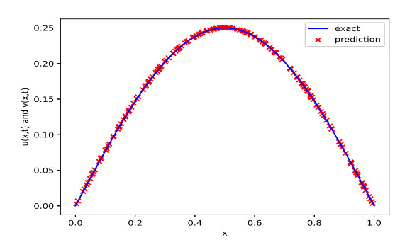
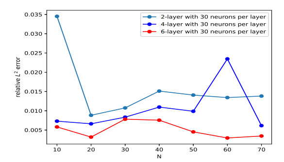
In order to conveniently observe the capability of our proposed method, Figure 7 shows the change in the trajectory of the predicted and exact solutions with respect to the space point x, where the parameters are set as N=20, Δα=1500, θ=1 and the network consists of 6 hidden layers with 50 neurons per layer. Figure 8 portrays the trajectory of relative L2 error with three different network architectures. Table 6 shows the impact of expanding depth or width of the network on the accuracy of the predicted solutions. Based on Figure 8 and Table 6, it is easy to observe that increasing the number of hidden layer plays a positive role in improving the accuracy of the predicted solutions.
 |
20 | 30 | 40 | 50 | 60 |
| 2 | 8.994465e-03 | 8.835675e-03 | 7.976196e-03 | 1.121301e-02 | 1.284193e-02 |
| 4 | 6.698531e-03 | 6.623791e-03 | 1.012124e-02 | 7.129064e-03 | 6.760145e-03 |
| 6 | 5.238653e-03 | 3.178300e-03 | 4.705057e-03 | 7.221552e-03 | 5.002096e-03 |
DownLoad:
CSV
The relative L2 error and CPU time obtained by the multi-output neural network and single output neural network schemes are presented in Table 7, where we select 200 collocation points in the given spatial domain by random sampling method and set N=10, θ=1 and Δα=1500. The error of the proposed multi-output neural network scheme is smaller than that of the single output neural network scheme. For this 1D system, the multi-output neural network scheme is more efficient than the single output neural network scheme.
| Neural network | Layers | Neurons | Relative L2 error | CPU time (s) |
| multi-output | 4 | 20 | 8.027377e-03 | 334.07 |
| 40 | 8.656712e-03 | 366.52 | ||
| 6 | 20 | 8.315435e-03 | 557.78 | |
| 40 | 6.788274e-03 | 601.19 | ||
| single output | 4 | 20 | 2.412753e-02 | 994.62 |
| 40 | 2.365781e-02 | 1317.16 | ||
| 6 | 20 | 2.428662e-02 | 1344.76 | |
| 40 | 2.139562e-02 | 1795.75 |
DownLoad:
CSV
Example 4.
Now we take space domain Ω=(0,1)×(0,1) and time interval J=(0,12]. Let ω(α)=Γ(3−α) and the exact solution u(x,y,t)=t2sin(πx)sin(πy). Then we arrive at the source term
| f(x,y,t)=2tsin(πx)sin(πy)+Γ(3)t(t−1)lntsin(πx)sin(πy)+2t2π2sin(πx)sin(πy)+4t2π4sin(πx)sin(πy)+(t2sin(πx)sin(πy))2. | (4.7) |
Here, we apply the training data set shown in Figure 5.
In order to more intuitively demonstrate the feasibility of our proposed method for solving this 2D system, Figure 9 shows the contour plot of u and |u−v|, where the training set consists of 900 collocation points and 120 boundary points selected by the equidistant uniform sampling method and the network is composed of 6 hidden layers with 20 neurons per layer.

From the behavior of relative L2 error in Figure 10, one can see that the accuracy of the predicted solutions with the fixed network first presents a increasing trend and then gradually presents a downward trend. This is because the approximation ability of neural network reaches saturation with the increase of grid points N. Table 8 shows the relative L2 error calculated by different network architectures. On the whole, the relative L2 error slightly decreases with expanding depth of the network, while it first slightly decreases and then increases with expanding width of the network. To show the precision and efficiency of the multi-output neural network scheme for this 2D system, the relative L2 error and CPU time obtained by the multi-output neural network and single output neural network schemes are shown in Table 9, where we select 40 boundary points and 200 collocation points in the given spatial domain by random sampling method and set N=10, θ=1 and Δα=1500. It illustrates that the multi-output neural network scheme is more accurate and efficient than the single output neural network scheme.
 } } |
20 | 30 | 40 | 50 | 60 |
| 2 | 7.593424e-02 | 4.556132e-02 | 2.926755e-02 | 5.850593e-02 | 4.956921e-02 |
| 4 | 3.716823e-02 | 2.498269e-02 | 3.388639e-02 | 4.073820e-02 | 5.282780e-02 |
| 6 | 2.690082e-02 | 3.039336e-02 | 2.769315e-02 | 4.331023e-02 | 6.456580e-02 |
DownLoad:
CSV
| Neural network | Layers | Neurons | Relative L2 error | CPU time (s) |
| multi-output | 4 | 20 | 4.549939e-02 | 345.03 |
| 40 | 5.847813e-02 | 339.46 | ||
| 6 | 20 | 5.680785e-02 | 466.02 | |
| 40 | 6.110534e-02 | 528.10 | ||
| single output | 4 | 20 | 1.455785e-01 | 902.99 |
| 40 | 1.330922e-01 | 1309.05 | ||
| 6 | 20 | 1.496581e-01 | 1469.85 | |
| 40 | 1.322566e-01 | 1990.96 |
DownLoad:
CSV
In this article, a multi-output physics informed neural network combined with the Crank-Nicolson scheme including the FBN-θ method and the composite numerical integral formula was constructed to solve 1D and 2D nonlinear time distributed-order models. The calculation process is described in detail. Numerical experiments are provided to prove the effectiveness and feasibility of our algorithm. Compared with the results calculated by a single output neural network combined with the FBN-θ method and the Crank-Nicolson scheme, one can clearly see that the proposed multi-output neural network scheme is more efficient and accurate. Moreover, some numerical methods, such as finite difference or finite element method, need to linearize the nonlinear term, which will give rise to extra costs. The process of linearization can be directly omitted by PINN. Further work will investigate the application of the proposed methodology in high-dimensional problems and practical problems [36,37,38,39,40].
The authors declare that they have not used Artificial Intelligence (AI) tools in the creation of this article.
The authors would like to thank the editor and all the anonymous referees for their valuable comments, which greatly improved the presentation of the article. This work is supported by the National Natural Science Foundation of China (12061053, 12161063), Natural Science Foundation of Inner Mongolia (2021MS01018), Young innovative talents project of Grassland Talents Project, Program for Innovative Research Team in Universities of Inner Mongolia Autonomous Region (NMGIRT2413, NMGIRT2207), and 2023 Postgraduate Research Innovation Project of Inner Mongolia (S20231026Z).
The authors declare that they have no conflict of interest.
| [1] | J. Yang, Q. H. Zhu, A local deep learning method for solving high order partial differential equtaions, arXiv: 2103.08915 [Preprint], (2021), [cited 2023 Nov 22]. Available from: https://doi.org/10.48550/arXiv.2103.08915 |
| [2] |
J. Q. Han, A. Jentzen, W. N. E, Solving high-dimensonal partial differential equations using deep learning, Proc. Natl. Acad. Sci. U.S.A., 115 (2018), 8505–8510. https://doi.org/10.1073/pnas.1718942115 doi: 10.1073/pnas.1718942115

|
| [3] |
Y. Li, Z. J. Zhou, S. H. Ying, DeLISA: Deep learning based iteration scheme approximation for solving PDEs, J. Comput. Phys., 451 (2022), 110884. https://doi.org/10.1016/j.jcp.2021.110884 doi: 10.1016/j.jcp.2021.110884
|
| [4] |
X. J. Xu, M. H. Chen, Discovery of subdiffusion problem with noisy data via deep learning, J. Sci. Comput., 92 (2022), 23. https://doi.org/10.1007/s10915-022-01879-8 doi: 10.1007/s10915-022-01879-8
|
| [5] |
M. Raissi, P. Perdikaris, G. E. Karniadakis, Physics-informend neural networks: A deep learning framework for solving forward and inverse problems involving nonlinear partial differential equations, J. Comput. Phys., 378 (2019), 686–707. https://doi.org/10.1016/j.jcp.2018.10.045 doi: 10.1016/j.jcp.2018.10.045
|
| [6] |
L. Yuan, Y. Q. Ni, X. Y. Deng, S. Hao, A-PINN: Auxiliary physics informed neural networks for forward and inverse problems of nonlinear integro-differential equations, J. Comput. Phys., 462 (2022), 111260. https://doi.org/10.1016/j.jcp.2022.111260 doi: 10.1016/j.jcp.2022.111260
|
| [7] |
S. N. Lin, Y. Chen, A two-stage physics-informed neural network method based on conserved quantities and applications in localized wave solutions, J. Comput. Phys., 457 (2022), 111053. https://doi.org/10.1016/j.jcp.2022.111053 doi: 10.1016/j.jcp.2022.111053
|
| [8] |
L. Yang, X. H. Meng, G. E. Karniadakis, B-PINNs: Bayesian physics-informed neural networks for forward and inverse PDE problems with noisy data, J. Comput. Phys., 425 (2021), 109913. https://doi.org/10.1016/j.jcp.2020.109913 doi: 10.1016/j.jcp.2020.109913
|
| [9] |
P. Peng, J. G. Pan, H. Xu, X. L. Feng, RPINNs: Rectified-physics informed neural networks for solving stationary partial differential equations, Comput. Fluids., 245 (2022), 105583. https://doi.org/10.1016/j.compfluid.2022.105583 doi: 10.1016/j.compfluid.2022.105583
|
| [10] |
E. Kharazmi, Z. Q. Zhang, G. E. Karniadakis, hp-VPINNs: Variational physics-informed neural networks with domain decomposition, Comput. Meth. Appl. Mech. Eng., 374 (2021), 113547. https://doi.org/10.1016/j.cma.2020.113547 doi: 10.1016/j.cma.2020.113547
|
| [11] |
Z. P. Mao, A. D. Jagtap, G. E. Karniadakis, Physics-informed neural networks for high-speed flows, Comput. Meth. Appl. Mech. Eng., 360 (2020), 112789. https://doi.org/10.1016/j.cma.2019.112789 doi: 10.1016/j.cma.2019.112789
|
| [12] |
S. Z. Cai, Z. C. Wang, S. F. Wang, P. Perdikaris, G. E. Karniadakis, Physics-informed neural networks for heat transfer problems, J. Heat Trans., 143 (2021), 060801. https://doi.org/10.1115/1.4050542 doi: 10.1115/1.4050542
|
| [13] |
G. F. Pang, L. Lu, G. E. Karniadakis, fPINNs: Fractional physics-informed neural networks, SIAM J. Sci. Comput., 41 (2019), A2603–A2626. https://doi.org/10.1137/18M12298 doi: 10.1137/18M12298
|
| [14] |
L. Guo, H. Wu, X. C. Yu, T. Zhou, Monte Carlo PINNs: deep learning approach for forward and inverse problems involving high dimensional fractional partial differential equations, Comput. Meth. Appl. Mech. Engrg., 400 (2022), 115523. https://doi.org/10.1016/j.cma.2022.115523 doi: 10.1016/j.cma.2022.115523
|
| [15] |
W. K. Liu, Y. Liu, H. Li, Time difference physics-informed neural network for fractional water wave models, Results Appl. Math., 17 (2023), 100347. https://doi.org/10.1016/j.rinam.2022.100347 doi: 10.1016/j.rinam.2022.100347
|
| [16] |
P. Gatto, J. S. Hesthaven, Numerical approximation of the fractional laplacian via hp-finite elements, with an application to image denoising, J. Sci. Comput., 65 (2015), 249–270. https://doi.org/10.1007/s10915-014-9959-1 doi: 10.1007/s10915-014-9959-1
|
| [17] |
E. Barkai, R. Metzler, J. Klafter, From continuous time random walks to the fractional Fokker-Planck equation, Phys. Rev. E, 61 (2000), 132–138. https://doi.org/10.1103/PhysRevE.61.132 doi: 10.1103/PhysRevE.61.132
|
| [18] |
L. Feng, F. Liu, I. Turner, L. Zheng, Novel numerical analysis of multi-term time fractional viscoelastic non-Newtonian fluid models for simulating unsteady MHD Couette flow of a generalized Oldroyd-B fluid, Frac. Calc. Appl. Anal., 21 (2018), 1073–1103. https://doi.org/10.1515/fca-2018-0058 doi: 10.1515/fca-2018-0058
|
| [19] |
S. Vong, Z. B. Wang, A compact difference scheme for a two dimensional fractional Klein-Gordon equation with Neumann boundary conditions, J. Comput. Phys., 274 (2014), 268–282. https://doi.org/10.1016/j.jcp.2014.06.022 doi: 10.1016/j.jcp.2014.06.022
|
| [20] |
G. H. Gao, A. A. Alikhanov, Z. Z. Sun, The temporal second order difference schemes based on the interpolation approximation foe solving the time multi-term and distributed-order fractional sub-diffusion equations, J. Sci. Comput., 73 (2017), 93–121. https://doi.org/10.1007/s10915-017-0407-x doi: 10.1007/s10915-017-0407-x
|
| [21] |
H. Y. Jian, T. Z. Huang, X. M. Gu, X. L. Zhao, Y. L. Zhao, Fast second-order implicit difference schemes for time distributed-order and Riesz space fractional diffusion-wave equations, Comput. Math. Appl., 94 (2021), 136–154. https://doi.org/10.1016/j.camwa.2021.05.003 doi: 10.1016/j.camwa.2021.05.003
|
| [22] |
J. Li, F. Liu, L. Feng, I. Turner, A novel finite volume method for the Riesz space distributed-order advection-diffusion equation, Appl. Math. Model., 46 (2017), 536–553. https://doi.org/10.1016/j.apm.2017.01.065 doi: 10.1016/j.apm.2017.01.065
|
| [23] |
C. Wen, Y. Liu, B. L. Yin, H. Li, J. F. Wang, Fast second-order time two-mesh mixed finite element method for a nonlinear distributed-order sub-diffusion model, Numer. Algor., 88 (2021), 523–553. https://doi.org/10.1007/s11075-020-01048-8 doi: 10.1007/s11075-020-01048-8
|
| [24] |
S. Guo, L. Mei, Z. Zhang, Y. Jiang, Finite difference/spectral-Galerkin method for a two-dimensional distributed-order time-space fractional reaction-diffusion equation, Appl. Math. Lett., 85 (2018), 157–163. https://doi.org/10.1016/j.aml.2018.06.005 doi: 10.1016/j.aml.2018.06.005
|
| [25] |
H. Zhang, F. Liu, X. Jiang, F. Zeng, I. Turner, A Crank-Nicolson ADI Galerkin-Legendre spectral method for the two-dimensional Riesz space distributed-order advection-diffusion equation, Comput. Math. Appl., 76 (2018), 2460–2476. https://doi.org/10.1016/j.camwa.2018.08.042 doi: 10.1016/j.camwa.2018.08.042
|
| [26] |
M. H. Ran, C. J. Zhang, New compact difference scheme for solving the fourth-order time fractional sub-diffusion equation of the distributed order, Appl. Numer. Math., 129 (2018), 58–70. https://doi.org/10.1016/j.apnum.2018.03.005 doi: 10.1016/j.apnum.2018.03.005
|
| [27] |
M. F. Fei, C. M. Huang, Galerkin-Legendre spectral method for the distributed-order time fractional fourth-order partial differential equation, Int. J. Comput. Math., 97 (2020), 1183–1196. https://doi.org/10.1080/00207160.2019.1608968 doi: 10.1080/00207160.2019.1608968
|
| [28] |
F. Fakhar-Izadi, Fully Petrov-Galerkin spectral method for the distributed-order time-fractional fourth-order partial differential equation, Eng. Comput., 37 (2021), 2707–2716. https://doi.org/10.1007/s00366-020-00968-2 doi: 10.1007/s00366-020-00968-2
|
| [29] |
K. Diethelm, N. J. Ford, Numerical analysis for distributed-order differential equations, J. Comput. Appl. Math., 225 (2009), 96–104. https://doi.org/10.1016/j.cam.2008.07.018 doi: 10.1016/j.cam.2008.07.018
|
| [30] |
K. Diethelm, N. J. Ford, Analysis of fractional differential equations, J. Math. Anal. Appl., 265 (2002), 229–248. https://doi.org/10.1006/jmaa.2000.7194 doi: 10.1006/jmaa.2000.7194
|
| [31] |
B. L. Yin, Y. Liu, H. Li, Z. M. Zhang, Finite element methods based on two families of second-order numerical formulas for the fractional Cable model with smooth solutions, J. Sci. Comput., 84 (2020), 2. https://doi.org/10.1007/s10915-020-01258-1 doi: 10.1007/s10915-020-01258-1
|
| [32] |
B. L. Yin, Y. Liu, H. Li, Z. M. Zhang, Two families of second-order fractional numerical formulas and applications to fractional differential equations, Fract. Calc. Appl. Anal., 26 (2023), 1842–1867. https://doi.org/10.1007/s13540-023-00172-1 doi: 10.1007/s13540-023-00172-1
|
| [33] |
Y. LeCun, Y. Bengio, G. Hinton, Deep learning, Nature, 521 (2015), 436–444. https://doi.org/10.1038/nature14539 doi: 10.1038/nature14539
|
| [34] |
H. M. Chen, O. Engkvist, Y. H. Wang, M. Olivecrona, T. Blaschke, The rise of deep learning in drug discovery, Drug Discov. Today, 23 (2018), 1241–1250. https://doi.org/10.1016/j.drudis.2018.01.039 doi: 10.1016/j.drudis.2018.01.039
|
| [35] |
Y. B. Yang, P. Perdikaris, Adversarial uncertainty quantification in physics-informed neural networks, J. Comput. Phys., 394 (2019), 136–152. https://doi.org/10.1016/j.jcp.2019.05.027 doi: 10.1016/j.jcp.2019.05.027
|
| [36] |
B. L. Yin, Y. Liu, H. Li, Z. M. Zhang, On discrete energy dissipation of Maxwell's equations in a Cole-Cole dispersive medium, J. Comput. Math., 41 (2023), 980–1002. https://doi.org/10.4208/jcm.2210-m2021-0257 doi: 10.4208/jcm.2210-m2021-0257
|
| [37] |
J. Li, Y. Huang, Y. Lin, Developing finite element methods for Maxwell's equations in a Cole-Cole dispersive medium, SIAM J. Sci. Comput., 33 (2011), 3153–3174. https://doi.org/10.1137/110827624 doi: 10.1137/110827624
|
| [38] |
W. Wang, H. X. Zhang, X. X. Jiang, X. H. Yang, A high-order and efficient numerical technique for the nonlocal neutron diffusion equation representing neutron transport in a nuclear reactor, Ann. Nucl. Energy., 195 (2024), 110163. https://doi.org/10.1016/j.anucene.2023.110163 doi: 10.1016/j.anucene.2023.110163
|
| [39] |
Q. Q. Tian, X. H. Yang, H. X. Zhang, D. Xu, An implicit robust numerical scheme with graded meshes for the modified Burgers model with nonlocal dynamic properties, Comput. Appl. Math., 42 (2023), 246. https://doi.org/10.1007/s40314-023-02373-z doi: 10.1007/s40314-023-02373-z
|
| [40] |
Z. Y. Zhou, H. X. Zhang, X. H. Yang, H1-norm error analysis of a robust ADI method on graded mesh for three-dimensional subdiffusion problems, Numer. Algor., (2023), 1–19. https://doi.org/10.1007/s11075-023-01676-w doi: 10.1007/s11075-023-01676-w
|
| 1. | Jiahuan He, Yang Liu, Hong Li, TDOR-MPINNs: Multi-output physics-informed neural networks based on time differential order reduction for solving coupled Klein–Gordon–Zakharov systems, 2024, 22, 25900374, 100462, 10.1016/j.rinam.2024.100462 |
Figures(10) / Tables(9)
Wenkai Liu, Yang Liu, Hong Li, Yining Yang. Multi-output physics-informed neural network for one- and two-dimensional nonlinear time distributed-order models[J]. Networks and Heterogeneous Media, 2023, 18(4): 1899-1918. doi: 10.3934/nhm.2023080

| Example | Optimizer | Learning rate | Iterations |
| 1 | Adam + L-BFGS | 0.001 | 20000 |
| 2 | Adam + L-BFGS | 0.001 | 20000 |
| 3 | Adam + L-BFGS | 0.001 | 20000 |
| 4 | L-BFGS | - | - |
DownLoad:
CSV
|
20 | 30 | 40 | 50 | 60 |
| 2 | 3.583482e-02 | 7.850782e-02 | 5.238403e-02 | 1.143600e-01 | 3.761048e-02 |
| 4 | 3.815002e-02 | 5.144618e-02 | 3.622479e-02 | 2.317038e-02 | 3.721057e-02 |
| 6 | 2.433509e-02 | 1.216386e-01 | 2.638224e-02 | 2.837553e-02 | 2.682958e-02 |
DownLoad:
CSV
| Neural network | Layers | Neurons | Relative L2 error | CPU time (s) |
| multi-output | 4 | 20 | 1.948281e-02 | 32.80 |
| 40 | 1.858120e-02 | 44.45 | ||
| 6 | 20 | 9.724722e-03 | 51.40 | |
| 40 | 1.024869e-02 | 65.88 | ||
| single output | 4 | 20 | 8.741336e-02 | 661.99 |
| 40 | 2.702814e-02 | 742.17 | ||
| 6 | 20 | 2.937448e-02 | 748.31 | |
| 40 | 2.278774e-02 | 840.09 |
DownLoad:
CSV
|
20 | 30 | 40 | 50 | 60 |
| 4 | 1.155984e-01 | 1.101123e-01 | 7.228454e-02 | 7.787707e-02 | 4.492646e-02 |
| 6 | 6.273340e-02 | 6.088659e-02 | 9.802474e-02 | 6.536637e-02 | 6.245142e-02 |
| 8 | 6.163051e-02 | 7.424834e-02 | 6.844676e-02 | 5.500003e-02 | 5.169303e-02 |
DownLoad:
CSV
| Neural network | Layers | Neurons | Relative L2 error | CPU time (s) |
| multi-output | 4 | 20 | 1.080369e-01 | 52.84 |
| 40 | 7.472573e-02 | 66.05 | ||
| 6 | 20 | 6.654115e-02 | 72.71 | |
| 40 | 7.937601e-02 | 93.77 | ||
| single output | 4 | 20 | 3.443264e-01 | 731.22 |
| 40 | 7.054495e-01 | 728.11 | ||
| 6 | 20 | 2.636401e-01 | 772.08 | |
| 40 | 1.410780e-01 | 892.94 |
DownLoad:
CSV
|
20 | 30 | 40 | 50 | 60 |
| 2 | 8.994465e-03 | 8.835675e-03 | 7.976196e-03 | 1.121301e-02 | 1.284193e-02 |
| 4 | 6.698531e-03 | 6.623791e-03 | 1.012124e-02 | 7.129064e-03 | 6.760145e-03 |
| 6 | 5.238653e-03 | 3.178300e-03 | 4.705057e-03 | 7.221552e-03 | 5.002096e-03 |
DownLoad:
CSV
| Neural network | Layers | Neurons | Relative L2 error | CPU time (s) |
| multi-output | 4 | 20 | 8.027377e-03 | 334.07 |
| 40 | 8.656712e-03 | 366.52 | ||
| 6 | 20 | 8.315435e-03 | 557.78 | |
| 40 | 6.788274e-03 | 601.19 | ||
| single output | 4 | 20 | 2.412753e-02 | 994.62 |
| 40 | 2.365781e-02 | 1317.16 | ||
| 6 | 20 | 2.428662e-02 | 1344.76 | |
| 40 | 2.139562e-02 | 1795.75 |
DownLoad:
CSV
| } |
20 | 30 | 40 | 50 | 60 |
| 2 | 7.593424e-02 | 4.556132e-02 | 2.926755e-02 | 5.850593e-02 | 4.956921e-02 |
| 4 | 3.716823e-02 | 2.498269e-02 | 3.388639e-02 | 4.073820e-02 | 5.282780e-02 |
| 6 | 2.690082e-02 | 3.039336e-02 | 2.769315e-02 | 4.331023e-02 | 6.456580e-02 |
DownLoad:
CSV
| Neural network | Layers | Neurons | Relative L2 error | CPU time (s) |
| multi-output | 4 | 20 | 4.549939e-02 | 345.03 |
| 40 | 5.847813e-02 | 339.46 | ||
| 6 | 20 | 5.680785e-02 | 466.02 | |
| 40 | 6.110534e-02 | 528.10 | ||
| single output | 4 | 20 | 1.455785e-01 | 902.99 |
| 40 | 1.330922e-01 | 1309.05 | ||
| 6 | 20 | 1.496581e-01 | 1469.85 | |
| 40 | 1.322566e-01 | 1990.96 |
DownLoad:
CSV
| Example | Optimizer | Learning rate | Iterations |
| 1 | Adam + L-BFGS | 0.001 | 20000 |
| 2 | Adam + L-BFGS | 0.001 | 20000 |
| 3 | Adam + L-BFGS | 0.001 | 20000 |
| 4 | L-BFGS | - | - |
|
20 | 30 | 40 | 50 | 60 |
| 2 | 3.583482e-02 | 7.850782e-02 | 5.238403e-02 | 1.143600e-01 | 3.761048e-02 |
| 4 | 3.815002e-02 | 5.144618e-02 | 3.622479e-02 | 2.317038e-02 | 3.721057e-02 |
| 6 | 2.433509e-02 | 1.216386e-01 | 2.638224e-02 | 2.837553e-02 | 2.682958e-02 |
| Neural network | Layers | Neurons | Relative L2 error | CPU time (s) |
| multi-output | 4 | 20 | 1.948281e-02 | 32.80 |
| 40 | 1.858120e-02 | 44.45 | ||
| 6 | 20 | 9.724722e-03 | 51.40 | |
| 40 | 1.024869e-02 | 65.88 | ||
| single output | 4 | 20 | 8.741336e-02 | 661.99 |
| 40 | 2.702814e-02 | 742.17 | ||
| 6 | 20 | 2.937448e-02 | 748.31 | |
| 40 | 2.278774e-02 | 840.09 |
|
20 | 30 | 40 | 50 | 60 |
| 4 | 1.155984e-01 | 1.101123e-01 | 7.228454e-02 | 7.787707e-02 | 4.492646e-02 |
| 6 | 6.273340e-02 | 6.088659e-02 | 9.802474e-02 | 6.536637e-02 | 6.245142e-02 |
| 8 | 6.163051e-02 | 7.424834e-02 | 6.844676e-02 | 5.500003e-02 | 5.169303e-02 |
| Neural network | Layers | Neurons | Relative L2 error | CPU time (s) |
| multi-output | 4 | 20 | 1.080369e-01 | 52.84 |
| 40 | 7.472573e-02 | 66.05 | ||
| 6 | 20 | 6.654115e-02 | 72.71 | |
| 40 | 7.937601e-02 | 93.77 | ||
| single output | 4 | 20 | 3.443264e-01 | 731.22 |
| 40 | 7.054495e-01 | 728.11 | ||
| 6 | 20 | 2.636401e-01 | 772.08 | |
| 40 | 1.410780e-01 | 892.94 |
|
20 | 30 | 40 | 50 | 60 |
| 2 | 8.994465e-03 | 8.835675e-03 | 7.976196e-03 | 1.121301e-02 | 1.284193e-02 |
| 4 | 6.698531e-03 | 6.623791e-03 | 1.012124e-02 | 7.129064e-03 | 6.760145e-03 |
| 6 | 5.238653e-03 | 3.178300e-03 | 4.705057e-03 | 7.221552e-03 | 5.002096e-03 |
| Neural network | Layers | Neurons | Relative L2 error | CPU time (s) |
| multi-output | 4 | 20 | 8.027377e-03 | 334.07 |
| 40 | 8.656712e-03 | 366.52 | ||
| 6 | 20 | 8.315435e-03 | 557.78 | |
| 40 | 6.788274e-03 | 601.19 | ||
| single output | 4 | 20 | 2.412753e-02 | 994.62 |
| 40 | 2.365781e-02 | 1317.16 | ||
| 6 | 20 | 2.428662e-02 | 1344.76 | |
| 40 | 2.139562e-02 | 1795.75 |
| } |
20 | 30 | 40 | 50 | 60 |
| 2 | 7.593424e-02 | 4.556132e-02 | 2.926755e-02 | 5.850593e-02 | 4.956921e-02 |
| 4 | 3.716823e-02 | 2.498269e-02 | 3.388639e-02 | 4.073820e-02 | 5.282780e-02 |
| 6 | 2.690082e-02 | 3.039336e-02 | 2.769315e-02 | 4.331023e-02 | 6.456580e-02 |
| Neural network | Layers | Neurons | Relative L2 error | CPU time (s) |
| multi-output | 4 | 20 | 4.549939e-02 | 345.03 |
| 40 | 5.847813e-02 | 339.46 | ||
| 6 | 20 | 5.680785e-02 | 466.02 | |
| 40 | 6.110534e-02 | 528.10 | ||
| single output | 4 | 20 | 1.455785e-01 | 902.99 |
| 40 | 1.330922e-01 | 1309.05 | ||
| 6 | 20 | 1.496581e-01 | 1469.85 | |
| 40 | 1.322566e-01 | 1990.96 |
