Robust network formation with biological applications

1.   Introduction

In this paper we focus on the discrete graph model introduced by Hu and Cai ^[14] and further studied in ^[2,6,9,15] which describes optimal transportation networks in a primarily biological context. Typical examples are leaf venation in plants, mammalian circulatory systems that convey nutrients to the body through blood circulation, or neural networks that transport electric charge. Understanding the properties of optimal transportation networks and mechanisms of their development, function, and adaptation has been the subject of an active field of research, see, e.g., ^[4,7,24,30].

Mathematical modeling of transportation networks is traditionally based on the frameworks of mathematical graph theory and discrete energy optimization. The model studied in ^[14] falls into this category, being formulated as an energy functional depending on edge conductivities of a given undirected discrete graph, constrained by a local mass conservation law. The mass conservation law is imposed in terms of a linear system of equations for the material pressures known as Kirchhoff law. The energy consists of a pumping term, describing the kinetic energy of the material flow through the network, and a metabolic term, which reflects the biological motivation of the model. The metabolic term is a function of the edge conductivities and is assumed to be of power-law form, with exponent $\gamma > 0$. For biological applications, one usually assumes that $\gamma\in [1/2, 1]$. We note that for $\gamma < 1$ the energy functional is nonconvex, while for $\gamma = 1$ it is convex, and for $\gamma > 1$ it is strictly convex ^[14].

The first goal of this paper is to provide two new results regarding the (local) minimizers of the energy. In particular, it has been shown ^[6] that for $\gamma < 1$, each minimizer of the energy is a loop-free graph, i.e., an undirected graph where each pair of nodes is connected by at most one path. Here we show the complementary claim, namely, that if $\gamma < 1$, every admissible loop-free graph represents a local minimizer of the energy. The term "admissible" refers to a graph for which the Kirchhoff law is solvable when all edges with zero conductivity are treated as void (nonexistent). Moreover, we show that for $\gamma = 1$ every (local) minimizer is a set containing a loop-free graph.

The second goal of this paper is to incorporate the concept of robustness into the model ^[14]. In particular, the fact that, for biological applications where $\gamma\leq 1$, the energy minimizers are loop-free, does not correspond to the transportation networks observed in most real organisms, where typically (many) loops are present. For a striking example of a highly redundant pattern in leaf venation, we refer to [17, Figure 1]. There, the authors assert that the high redundancy of paths from the leaf base to any point on the leaf surface might be very advantageous with regard to local damages, i.e., they promote robustness of the transportation network against the removal of edges. We therefore propose to incorporate the robustness aspect into the discrete model ^[14] by extending the energy functional by a term that measures the connectivity of the network.

The concept of network robustness (or resilience) is usually defined as the ability of a network to maintain its function when subjected to disturbances or attacks ^[1,27]. In our paper, we understand the term robustness as the ability of the network to withstand disturbance of its connectivity through the removal of edges. A generally accepted measure of connectivity of a discrete graph is the Cheeger constant ^[19,21], also called the isoperimetric number or minimum cut. Loosely speaking, the Cheeger constant is a numerical measure of whether or not a graph has a "bottleneck", i.e., a small subset of edges whose removal destroys the connectivity of the graph. The Cheeger constant is strictly positive if and only if the underlying (undirected) graph is connected. Graphs with a small (but positive) Cheeger constant have a "bottleneck", in the sense that there are two "large" sets of vertices with "few" links (edges) between them. On the other hand, the Cheeger constant is "large" if any possible division of the vertex set into two subsets has "many" links between those two subsets. The fundamental problem is that the calculation of the isoperimetric number of graphs with multiple edges is NP hard ^[19]. To circumvent this issue and to obtain a practically tractable optimization problem, we propose to replace it by a related quantity, the algebraic connectivity, also called the Fiedler number ^[8]. This is defined as the second smallest eigenvalue of the matrix Laplacian of the connectivity matrix of the graph; for a connected graph, this is the smallest nonzero eigenvalue. The Fiedler number is another generally accepted measure of network robustness ^[18,21], and is related to the Cheeger constant by the well-known Cheeger inequalities ^[19]. These state that the isoperimetric number is bounded from below by one half of the Fiedler number. Consequently, knowing that a given graph is "well-connected" due to a sufficiently large value of its Fiedler number guarantees robustness also in terms of its Cheeger constant.

In this paper, we take into account the connectivity of the graph in terms of the Fiedler number calculated from the weighted adjacency matrix, with weights equal to the edge conductivities. This is motivated by the fact that, if a certain transport path is severed due to the removal of some edges, then the "alternative" (backup) path should have enough transport capacity, i.e., high enough conductivity. The Fiedler number is then a Lipschitz continuous function of the edge conductivities. Moreover, as long as it represents a simple eigenvalue (i.e., of multiplicity one) of the matrix Laplacian, it is differentiable with respect to the conductivities.

We thus formulate a new energy functional, where a multiple of the Fiedler number is subtracted from the pumping (kinetic) and metabolic energy terms. We then present two toy examples demonstrating how the modified energy functional enforces connectivity of the optimal transportation network. Moreover, since the Fiedler number is a concave function of the edge conductivities, the problem remains convex as long as the metabolic exponent $\gamma\geq 1$. The convexity and Lipschitz continuity of the modified energy functional facilitate the application of the projected subgradient method for its numerical minimization. We then present results of two numerical experiments, further documenting how the connectivity of the graph and its energy expenditure grow with increasing relative weight of the Fiedler number in the modified energy functional.

This paper is organized as follows. In Section 2, we describe the discrete network formation model of Hu and Cai ^[14] and establish some of its fundamental properties (convexity and boundedness of the kinetic energy). We also introduce the matrix Laplacian and Fiedler number of the graph. In Section 3, we provide results about the structure of optimal transportation networks in the cases $\gamma < 1$ and $\gamma = 1$. In Section 4, we extend the energy functional such that it also accounts for robustness of the transportation network in terms of the Fiedler number of the weighted graph. We then establish basic mathematical properties of the modified functional with $\gamma = 1$, namely, boundedness from below, coercivity, and convexity. We also provide insights into the new model by studying two toy examples. Finally, in Section 5, we implement the projected subgradient method to find global minimizers of the modified functional numerically. We present two examples where we demonstrate how the structure of the optimal graphs depends on the required robustness of the network.

2.   The model

The discrete network formation model introduced by Hu and Cai ^[14] is posed on a prescribed undirected connected graph $G = (V, E)$, consisting of a finite set of vertices $V$, also called nodes, and a finite set of edges $E$. The number of vertices shall be denoted by $| V|$ in the sequel. Any pair of vertices is connected by at most one edge and no vertex is not connected to itself (i.e., the graph does not contain "self-loops"). The edge between vertices $i\in V$ and $j\in V$ is denoted by $(i, j)\in E$. Since the graph is undirected, we refer by $(i, j)$ and $(j, i)$ to the same edge. For each edge $(i, j)\in E$ of the graph $G$, we prescribe its length $L_{ij} = L_{ji} > 0$.

Throughout the paper, we assume that the graph $G$ is connected, i.e., that every pair of vertices in $V$ is connected by an undirected path (sequence of edges) in $E$.

We treat the graph as a transportation structure, and in each vertex $i\in V$ we have the pressure $P_i\in{\mathbb{R}}$ of the medium flowing through the network. The oriented flux (flow rate) from vertex $i\in V$ to $j\in V$ is denoted by $Q_{ij}$; obviously, we have the antisymmetry $Q_{ij} = -Q_{ji}$. For biological networks, the Reynolds number of the flow is typically small and the flow is predominantly in the laminar (Poiseuille) regime. Then the flow rate between vertices $i\in V$ and $j\in V$ along the edge $(i, j)\in E$ is proportional to the conductance $C_{ij}\geq 0$ of the edge and the pressure drop $P_i-P_j$,

The local mass conservation in each vertex is expressed in terms of the Kirchhoff law

Here $N(i)$ denotes the set of vertices connected to $i\in V$ through an edge, i.e., $N(i) : = \{ j\in V; \, (i, j)\in E \}.$ Moreover, $S = (S_i)_{i\in V}$ is the strength of the flow source ($S_i > 0$) or sink ($S_i < 0$) at vertex $i$, which has to be prescribed as a datum to the model. Given the matrix of nonnegative conductivities $C = (C_{ij})_{(i, j)\in E}$ and the prescribed positive lengths $L = (L_{ij})_{(i, j)\in E}$, the Kirchhoff law (2.2) is a linear system of equations for the vector of pressures $P = (P_i)_{i\in V}$. Clearly, a necessary condition for the solvability of (2.2) is the global mass conservation $S\in{\mathbb{R}}^{|V|}_0$, where here and in the sequel we denote

Remark 1 If $C$ is the adjacency matrix of a weighted connected graph, then the solution $P$ of Eq (2.2) always exists and is unique up to an additive constant. Although $E$ itself is connected, $C$ might be supported on a proper subset of $E$ and may therefore correspond to a disconnected graph; we then shortly say that $C$ is disconnected. In this case, the solution of (2.2) may not exist or, if it exists, it is not unique (up to an additive constant), as demonstrated in Example 2 in Appendix A. In the case when $C$ is disconnected and (2.2) is solvable, we denote the connected components of $C$ by $\Gamma_1, \dots, \Gamma_n$ and observe that $\sum_{j\in \Gamma_k}S_j = 0$ for every $1\le k\le n$. Then $P$ is uniquely defined up to $n$ additive constants, one for every component $\Gamma_k$. Therefore, the matrix of fluxes $Q$ is still uniquely defined by Eq (2.1). On the other hand, if Eq (2.2) is not solvable, then $C$ is disconnected.

The conductivities $C_{ij} = C_{ji} \geq 0$ of the edges are subject to an energy optimization process. Hu and Cai ^[14] proposed an energy cost functional consisting of a pumping power term and a metabolic cost term. According to Joule's law, the power (kinetic energy) needed to pump material through an edge $(i, j)\in E$ is proportional to the pressure drop $P_i-P_j$ and the flow rate $Q_{ij}$ along the edge, i.e.,

The metabolic cost of maintaining the edge is assumed to be proportional to its length $L_{ij}$ and the power of its conductivity $C_{ij}^{\gamma}$, with an exponent $\gamma > 0$. For instance, in blood vessels, the metabolic cost is proportional to the cross-section area of the vessel ^[20]. Modeling the blood flow by Hagen-Poiseuille's law, the conductivity is proportional to the square of the cross-section area, implying $\gamma = 1/2$ for blood vessel systems. For models of leaf venation, the material cost is proportional to the number of small tubes, which is proportional to $C_{ij}$, and the metabolic cost is due to the effective loss of the photosynthetic power at the area of the venation cells, which is proportional to $C_{ij}^{1/2}$. Consequently, the effective value of $\gamma$ typically used in models of leaf venation lies between $1/2$ and $1$, see, e.g., ^[15]. The energy cost functional is thus given by

where $Q_{ij} = Q_{ij}[C]$ is given by Eq (2.1) with pressures calculated from the Kirchhoff law (2.2), and $\nu > 0$ is the so-called metabolic coefficient. Note that every edge of the graph $G$ is counted exactly once in the above sum, i.e., we identify each edge $(i, j)$ with $(j, i)$ and the energy can also be written as

where we set $L_{ij} : = 0$ whenever $(i, j)\notin E$. If $C$ is such that the linear system (2.2) is not solvable, we formally set ${\mathcal{E}}[C]: = +\infty$. In the sequel, we shall sometimes address the kinetic (pumping) and metabolic parts of the energy separately. For this purpose, we denote

In order to find the optimal transportation structure for a given vector of sources and sinks $S\in{\mathbb{R}}^{|V|}_0$, one needs to find the (global) minimum of the energy functional (2.4), coupled to the Kirchhoff law (2.1) and (2.2). The energy functional is to be minimized over the convex set $\mathcal{C}$ of symmetric matrices with nonnegative elements,

If the optimal solution has $C_{ij} = C_{ij} = 0$ for any $(i, j)\in E$, then the corresponding edge $(i, j)$ is considered nonexistent. We collected some basic mathematical properties of the functional ${\mathcal{E}} = {\mathcal{E}}[C]$ in Appendix A. An important property in the context of the optimization task (2.1)–(2.4) is the convexity of the problem.

Proposition 1. The energy functional (2.4), constrained by the Kirchhoff law (2.1) and (2.2), is strictly convex for $\gamma > 1$ and convex for $\gamma = 1$.

This result is not new, see for instance ^[10,11] for an analogous result for the continuum version of the problem. For the sake of the reader, we offer its proof for the discrete model (2.1)–(2.4) in the Appendix (Lemma 8). Convexity of the functional shall be instrumental in employing the projected subgradient method in Section 5.

2.1.   Matrix Laplacian and Fiedler number

Definition 1. For any $C\in \mathcal{C}$, we define the matrix Laplacian ${\mathcal{L}}[C]$ as

where $D$ is the diagonal matrix of row/column sums of $C$ (recall that $C\in \mathcal{C}$ is symmetric). For simplicity, we shall often write just ${\mathcal{L}}$ instead of ${\mathcal{L}}[C]$.

With this definition, we can express the Kirchhoff law (2.2) in the form

where we introduce the matrix $\widetilde C_{ij} : = C_{ij}/L_{ij}$, with $\widetilde C_{ij} : = 0$ if $L_{ij} = 0$ (recall that $L_{ij} = 0$ means that $(i, j)\notin E$ and, consequently, $C_{ij} = 0$). Moreover, we denoted $P = (P_i)_{i\in V}$ the vector of pressures and $S = (S_i)_{i\in V}$ the vector of sources and sinks.

We also note that if $P$ is a solution of (2.7), then an easy calculation gives the following expression for the kinetic energy (2.5),

Definition 2. The Fiedler number ${\mathfrak{f}}[C]$ of a matrix $C\in \mathcal{C}$ is the second smallest eigenvalue of the matrix Laplacian ${\mathcal{L}}[C]$, where multiple eigenvalues are counted separately ^[8].

2.2.   An upper bound on the kinetic energy

Lemma 1. Let $0 \neq S \in R_0^{|V|}$. For any $C\in \mathcal{C}$, we have

where ${{\mathcal{E}}_{\mathrm{kin}}}[C]$ is defined in Eq (2.5) and $\widetilde C_{ij} : = C_{ij}/L_{ij}$, with $\widetilde C_{ij} : = 0$ if $L_{ij} = 0$. Here and in the sequel, $\left\| {S} \right\|$ denotes the $\ell^2$-norm of the vector $S$.

Proof. For the case when $C\in \mathcal{C}$ is such that the Kirchhoff law (2.7) is not solvable, we have set ${{\mathcal{E}}_{\mathrm{kin}}}[C] = +\infty$. But then the graph composed of edges $(i, j)$ with $C_{ij} > 0$ is not connected, see Remark 1, thus ${\mathfrak{f}}[C] = 0$ and (2.9) holds.

Let us now fix $C\in \mathcal{C}$ such that the Kirchhoff law (2.7) admits a solution $P\in{\mathbb{R}}^{|V|}$. Since $P$ can be shifted by an additive constant, we choose $P\in{\mathbb{R}}^{|V|}_0$. Therefore, denoting $\mathbf{1} : = (1, \ldots, 1)\in{\mathbb{R}}^{|V|}$, we have $P^T \mathbf{1} = 0$. The Courant-Fisher (minimax) theorem ^[22] gives

Consequently,

Taking a scalar product of Eq (2.7) with $P$ and applying the Cauchy-Schwartz and Young inequalities yields

Combining this with Eq (2.11), we obtain

and we conclude by using Eq (2.8). □

3.   The structure of optimal transportation networks for $\gamma\leq 1$

In this section, we shall provide results about the structure of optimal transportation networks for $\gamma < 1$ and $\gamma = 1$. Let us recall that we assume the graph $G = (V, E)$ to be connected.

3.1.   Trees are local minimizers for $\gamma < 1$

In [6, Theorem 2.1], the authors proved that every global minimizer of the energy functional (2.4) with $\gamma < 1$, constrained by the Kirchhoff law (2.1) and (2.2), is loop-free (again, we remind that edges with zero conductivities are treated as nonexistent). By a very slight modification of the proof, one can extend the claim to local minimizers. Here we prove the opposite claim, namely, that for $\gamma < 1$ and every spanning tree of the connected graph $(V, E)$, we can find a set of conductivities $C\in \mathcal{C}$ supported on the spanning tree which is a local minimizer of the constrained energy.

Theorem 1. Let $\gamma < 1$ and let $(V, \tilde E)$, $\tilde E \subseteq E$, be a spanning tree of the connected graph $(V, E)$. Then there exists a set of conductivities $\tilde C\in \mathcal{C}$, supported on $\tilde E$, which is a local minimizer of the energy (2.4) constrained by the Kirchhoff law (2.1) and (2.2), on the set $\mathcal{C}$.

Proof. We observe that since $(V, \tilde E)$ is a tree, the fluxes $\tilde Q_{ij}$ for $(i, j)\in\tilde E$ are uniquely determined by $S$. Indeed, for any edge $(i, j)\in\tilde E$, there is a unique split of the vertices into two disjoint sets $V^{(i)}$, $V^{(j)}$ such that nodes from $V^{(i)}$ are connected to $i$ by paths in $\tilde E \setminus \{(i, j)\}$, and analogously for nodes in $V^{(j)}$. By the local mass conservation, the flux through $(i, j)$ is then given by

Once we identified the fluxes by the above prescription, we construct the conductivities $\tilde C\in \mathcal{C}$ as follows,

Obviously, $\tilde C$ is supported on $\tilde E$. We now claim that $\tilde C$ represents a local minimizer of the energy (2.4) constrained by the Kirchhoff law (2.1) and (2.2) on the set $\mathcal{C}$.

Let us first observe that since $(V, \tilde E)$ is connected, the Kirchhoff law (2.2) admits a solution $\tilde P\in{\mathbb{R}}^{|V|}$. Clearly, the fluxes $\tilde Q_{ij}$ constructed in (3.1) verify the relation (2.1). Moreover, we recall the formula [9, Lemma 2.1] for the derivative

Then, by Eq (3.2), we have

Moreover, using Eq (2.1), we recast Eq (3.3) as

which gives

where the partial derivative is taken from the right, i.e., as $\tilde C_{ij}\to 0+$. Since $\tilde C\in \mathcal{C}$ is a unique element of $\mathcal{C}$ with these properties, we conclude that it is a local minimizer of ${\mathcal{E}} = {\mathcal{E}}[C]$ on $\mathcal{C}$. □

Remark 2. Combining the claims of Theorem 1 and [6, Theorem 2.1] implies that the set of local minimizers of the energy functional (2.4) with $\gamma < 1$ is the set of spanning trees of the graph $(V, E)$. Consequently, a possible way to find the global minimizer is to search the set of spanning trees and identify the one with the smallest value of the energy ${\mathcal{E}} = {\mathcal{E}}[C]$. The value of the energy for any given tree is calculated using the procedure described in the proof of Theorem 1. Clearly, this approach quickly turns computationally infeasible with the growing size of the graph. For instance, the number of spanning trees for a complete graph with $| V|$ nodes is $| V|^{| V|-2}$ by Cayley's formula. For planar graphs, the number of possible spanning trees grows exponentially, see, e.g., ^[5].

3.2.   The structure of the set of minimizers for $\gamma=1$

In this section, we consider the energy functional ${\mathcal{E}} = {\mathcal{E}}[C]$ with $\gamma = 1$. By Proposition 1, ${\mathcal{E}}$ is a convex function on $\mathcal{C}$ and, therefore, the set $M$ of its minimizers,

is a closed convex subset of $\mathcal{C}$. Moreover, due to the coercivity

it is nonempty. Its structure is characterized by the following theorem.

Theorem 2. Let $\gamma = 1$ and let $M$ be defined by Eq (3.4). Then the extremal points of $M$ represent loop-free graphs, and vice-versa, the loop-free elements of $M$ are extremal points of $M$.

Proof. We first prove that the extremal points of $M$ represent loop-free graphs. Let $\tilde C\in M$. Since ${\mathcal{E}}[\tilde C] < +\infty$, the Kirchhoff law (2.2) admits a solution $\tilde P\in{\mathbb{R}}^{|V|}$. Formula (A.11) gives

If $\tilde C_{ij} > 0$ for some $(i, j)\in E$, we have $\frac{\partial {\mathcal{E}}[\tilde C]}{\partial\tilde C_{ij}} = 0$ and, consequently,

For contradiction, let us now assume that $\tilde C$ contains a loop, i.e., that there is a chain of edges

such that $\tilde C_{i_j, i_{j+1}} > 0$ for $j = 0, \dots, K-1$ (we count the indices modulo $K$, so $i_{K}\equiv i_0$). We also assume that ${\mathcal T}$ is the shortest loop, i.e., that all $i_0, \dots i_{K-1}$ are mutually different. By Eq (3.5), we know that $\tilde P_{i_j}\neq \tilde P_{i_{j+1}}$ and, with (2.1), the corresponding fluxes $\tilde Q_{i_j, i_{j+1}}$ are all nonvanishing.

We rewrite Eq (3.5) as

and sum these identities over $j = 0, \dots, K-1$ to obtain

We now perturb $\tilde Q$ by adding a circular flow along ${\mathcal T}.$ For $(i, j)\in E\setminus {\mathcal T}$ we set

while for $l = 0, \dots, K-1$,

with some $\varepsilon\neq 0$. Obviously, if $|\varepsilon|$ is small enough, we have $C\in \mathcal{C}.$ Also the local mass conservation $\sum_{j\in N(i)} Q_{ij}=S_i$ is verified for all $i\in V.$ Moreover, if $(i, j)\not\in {\mathcal T}$, then $Q_{ij}=C_{ij} \frac{\tilde P_i-\tilde P_j}{L_{ij}}$ remains true. On the other hand, for $(i_l, i_{l+1})\in{\mathcal T}$ we use Eqs (3.7) and (3.9) to get

Finally, using Eqs (3.5), (3.9), and (3.8) successively, we have

so that one more application of (3.5) gives

This immediately implies that ${\mathcal E}[C] = {\mathcal E}[\tilde C]$. It follows that if $\tilde C$ contains a loop, then it can be written as a convex combination of $C^{(+)}$ and, respectively, $C^{(-)}\in \mathcal{C}$, which are obtained from $\tilde C$ by taking (small) positive and, respectively, negative ${\varepsilon}$ in Eq (3.9). Therefore, $\tilde C$ is not an extremal point of $M$. This concludes the proof that all extremal points of $M$ are loop-free.

Let us now prove the converse claim, namely, that every loop-free element of $M$ is an extremal point. Let $C\in M$ be loop-free and assume, for contradiction, that $C$ can be written as $C = \alpha C^{(1)}+(1-\alpha)C^{(2)}$ for some $0 < \alpha < 1$ and $C^{(1)}, C^{(2)}\in M$. But then

which means that $C^{(1)}$ and $C^{(2)}$ are also loop-free. As ${\mathcal{E}}(C) = {\mathcal{E}}(C^{(1)}) = {\mathcal{E}}(C^{(2)}) < +\infty$, the Kirchhoff law (2.2) is solvable with $C$, $C^{(1)}$ and, respectively, $C^{(2)}$, and (2.1) gives the corresponding fluxes $Q$, $Q^{(1)}$ and, respectively, $Q^{(2)}$. As for loop-free networks the fluxes are uniquely determined by the sources/sinks $S$, we have $Q = Q^{(1)} = Q^{(2)}$ and, in turn, $C = C^{(1)} = C^{(2)}$. Hence, $C$ is an extremal point. □

4.   Introducing robustness

The Cheeger constant (also called the isoperimetric number) of a graph is a numerical measure of whether or not a graph has a "bottleneck". For $G = (V, E)$, its Cheeger constant ${\mathfrak{h}}(G)$ is defined as

where $\partial W \subset E$ denotes the set of edges having one end in $W$ and the other end in $V\setminus W$.

The Cheeger constant is strictly positive if and only if $G$ is a connected graph. Intuitively, if the Cheeger constant is small but positive, then there exists a "bottleneck", in the sense that there are two "large" sets of vertices with "few" links (edges) between them. The Cheeger constant is large if any possible division of the vertex set into two subsets has "many" links between those two subsets. In other words, it is a measure of resilience of the network against disturbance of the connectivity through the removal of edges.

In general, the calculation of the isoperimetric number of graphs with multiple edges is NP hard ^[19]. Consequently, we consider a related quantity, the algebraic connectivity, also called the Fiedler number, defined as the second smallest eigenvalue of the matrix Laplacian ${\mathcal{L}} = {\mathcal{L}}[A]$ of the adjacency matrix $A$. For a connected graph, which we assume throughout this paper, it is the smallest nonzero eigenvalue of ${\mathcal{L}}[A]$. The Fiedler number ${\mathfrak{f}}(G)$ is another classical measure of connectivity of the graph, or robustness with respect to edge removal. It is related to the isoperimetric number by the well-known Cheeger inequalities ^[19],

where $\Delta(G)$ is the maximum degree for the nodes in $G$.

In our paper, we shall work with the generalized Fiedler number ${\mathfrak{f}}[C]$, calculated as the second smallest eigenvalue of the weighted matrix Laplacian ${\mathcal{L}}[C]$ with weights given by the edge conductivities $C\in \mathcal{C}$. This reflects the modeling assumption that edges with higher conductivities contribute more to overall network robustness (for instance, because they may be more resilient against severing). Our idea is to modify the energy functional (2.4) to take robustness into account in terms of the generalized Fiedler number ${\mathfrak{f}}[C]$. Consequently, for $\mu > 0$ we introduce the modified energy functional ${\mathcal{F}} = {\mathcal{F}}[C]$,

where ${\mathcal{E}} = {\mathcal{E}}[C]$ is defined in (2.4) and

The reason for scaling the second term in (4.1) by ${\ell}$ is that the energy (2.4) is homogeneous with respect to the edge lengths, i.e., a multiplication of $L=(L_{ij})_{(i, j)\in E}$ by a positive factor leads to a rescaling of the value of the energy by the same factor. Consequently, the modified energy (4.1) has the same scaling property. The motivation for introducing the factor $\frac{|V|-1}{2}$ is clarified in Lemma 2 below.

Recalling that the model (2.1)–(2.4) bears relevance in biological applications as long as $\gamma\leq 1$, we consider the modified energy functional (4.1) exclusively with $\gamma = 1$ in the sequel. The reason for excluding the values $\gamma < 1$ is that ${\mathcal{F}} = {\mathcal{F}}[C]$ with $\mu > 0$ is then, in general, not bounded from below.

Example 1. Let us consider a complete graph with all edges of the same length, i.e., $L_{ij} = {\ell}$ for all $(i, j)\in E$. Moroever, for some $c > 0$, let us take $C_{ij} = c$ for all $(i, j)\in E$. Then we have ${\mathfrak{f}}[C] = c |V|$ and

Lemma 1 gives

with $\widetilde C_{ij} : = C_{ij}/L_{ij} = c/{\ell}$. Consequently, we readily have $\lim_{c\to+\infty} {\mathcal{F}}[C] = -\infty$ whenever $\gamma < 1$ and $\mu > 0$.

On the other hand, for $\gamma = 1$ we have the following Lemma establishing boundedness of ${\mathcal{F}} = {\mathcal{F}}[C]$ from below if $\mu\leq\nu$ and coercivity if $\mu < \nu$. It is a direct consequence of [8], Claim 3.5], which gives an upper bound on the value of the Fiedler number. We provide the complete proof here for the sake of the reader.

Lemma 2. Let $\gamma = 1$ and $\mu \leq \nu$. Then the modified energy functional ${\mathcal{F}} = {\mathcal{F}}[C]$, defined in Eq (4.1), satisfies

Moreover, if $\mu < \nu$, then ${\mathcal{F}} = {\mathcal{F}}[C]$ is coercive in the sense that there exists $\alpha > 0$ such that

Proof. Let ${\mathcal{L}}$ be the Laplacian matrix corresponding to $C\in \mathcal{C}$ and let ${\mathfrak{f}}[C]$ be the Fiedler number of $C$. We use the Courant-Fisher representation (2.10) of ${\mathfrak{f}}[C]$ in the form

We claim that the matrix

is positive semidefinite. Let us choose any vector $y\in{\mathbb{R}}^{|V|}$, then we have the decomposition $y = \alpha \mathbf{1} + \beta v$, where $v\perp\mathbf{1}$ and $\left\| {v} \right\| = 1$. Since, trivially, $\widetilde {\mathcal{L}} \mathbf{1} = \mathcal{O}$, where $\mathcal{O}$ denotes the zero vector in ${\mathbb{R}}^{|V|}$, we have

where the nonnegativity follows from Eq (4.5). Indeed, $\widetilde {\mathcal{L}}$ is positive semidefinite, and, consequently, all its diagonal elements are nonnegative. In particular,

so that

Therefore, using the convention $L_{ij} = C_{ij} = 0$ if $(i, j)\notin E$, we finally conclude that

with ${\ell} = \min_{(i, j)\in E} L_{ij} > 0$ as defined in Eq (4.2). For $\mu\leq\nu$ this immediately gives (4.3). Moreover, if $\mu < \nu$, then Eq (4.4) holds with $\alpha : = (\nu-\mu) \frac{{\ell}}{2} > 0$. □

Remark 3. The statement of Lemma 2 is optimal in the following sense: Considering again the setting from Example 1, we have

Consequently, $\lim_{c\to+\infty} {\mathcal{F}}[C] = 0$ if $\mu = \nu$, and $\lim_{c\to+\infty} {\mathcal{F}}[C] = -\infty$ if $\mu > \nu$.

Let us note that the idea of promoting robustness of the transportation network by means of the Fiedler number ${\mathfrak{f}}[C]$ can also be realized by minimizing (2.4) subject to (2.1) and (2.2) on the subset of $\mathcal{C}$ where ${\mathfrak{f}}[C]\geq \mu$, for a given $\mu > 0$. With this setting, the values of $\gamma < 1$ are perfectly admissible. We plan to explore this direction in a future work.

A fundamental property of the functional (4.1) with $\gamma = 1$ is its convexity.

Lemma 3. The functional (4.1) with $\gamma = 1$ is convex on the set $\mathcal{C}$.

Proof. We recast (4.5) as

Therefore, ${\mathfrak{f}}[C]$ is a minimum of linear functionals in $C$ and thus concave. The claim follows directly from the convexity of ${\mathcal{E}} = {\mathcal{E}}[C]$ with $\gamma = 1$ established in Proposition 1. □

Finally, we have the following trivial observation about monotonicity of the Fiedler number of the minimizers of (4.1) with respect to the values of $\mu\geq 0$.

Lemma 4. Fix $0 \leq \mu_1 \leq \mu_2$ and assume that $C^1$, and, respectively, $C^2\in \mathcal{C}$ are global minimizers of (4.1) on $\mathcal{C}$ with $\mu_1$ and, respectively, $\mu_2$. Then ${\mathfrak{f}}[C^1] \leq {\mathfrak{f}}[C^2]$.

Proof. For brevity, let us denote $\bar\mu_i : = \mu_i\, {\ell} \, \frac{|V|-1}{2}$ for $i = 1, 2$. According to the assumptions, we have

Adding these two inequalities gives

and since we have $\bar\mu_1 \leq \bar\mu_2$, the claim directly follows. □

Let us now present two toy models where, in a very simple setting, we are able to provide explicit results for the minimizers of (4.1) with $\gamma = 1$ and their dependence on the value of $\mu > 0$.

4.1.   Toy model: A triangle with sources/sinks $+1$, $-1$, $0$

Let us consider a network consisting of three nodes $V = \{0, 1, 2\}$ and three (unoriented) edges $E = \{(0, 1), (0, 2), (1, 2)\}$ of unit length. The sources and sinks are given by

Taking into account the symmetry of the problem, we denote $C_0$ the conductivity of the edge (0, 1), and $C_1$ the conductivity of the other two edges, (0, 2) and (1, 2). Moreover, let us denote $Q_0$ the flux from vertex 0 to vertex 1 through the edge (0, 1). Obviously, then the flux from vertex 0 to vertex 2 through the edge (0, 2) is $1-Q_0$ and the flux from vertex 1 to vertex 2 through the edge (1, 2) is $Q_0-1$. The Kirchhoff law yields, by a simple calculation,

Then the energy functional (2.4) with $\gamma = 1$ reads

with metabolic coefficient $\nu > 0$. The global minimizer $\bar C$ of $\mathcal{E}[C]$ is $\bar C_0 = 1/\sqrt\nu$, $\bar C_1 = 0$, with $\mathcal{E}[\bar C] = 2\sqrt\nu$. Obviously, with $\bar C_1 = 0$, only the edge $(0, 1)$ is present and, consequently, the graph is disconnected. However, since $S_2 = 0$, the Kirchhoff law (2.2) is solvable and the network still fulfills its task of transporting unit mass from node $0$ to node 1.

The eigenvalues of the matrix Laplacian of the corresponding weighted adjacency matrix are

Consequently, the Fiedler number is ${\mathfrak{f}}[C] = \min\{ 2C_0 + C_1, 3C_1 \}$ and the modified energy (4.1) reads

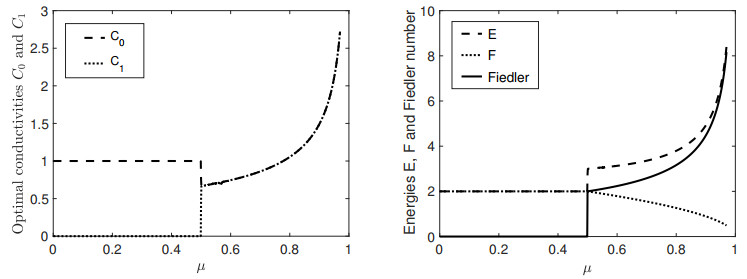
with $\mu \geq 0$. We note that due to the concavity of ${\mathfrak{f}}[C] = \min\{ 2C_0 + C_1, 3C_1 \}$ and strict (but non-uniform) convexity of the kinetic energy term $\frac{2}{2C_0 + C_1}$, the functional ${\mathcal{F}}[C]$ is non-uniformly strictly convex on the positive quadrant ${\mathbb{R}}^2_+$. Lemma 2 states that ${\mathcal{F}}[C]$ is bounded from below if $\mu\leq\nu$ and coercive if $\mu < \nu$. By inspecting the case $C_0 = C_1$, we see that this is also a necessary condition. In fact, for $\mu = \nu$, choosing $C_0 = C_1 = c$ with $c > 0$, we have ${\mathcal{F}}[C] = \frac{2}{3c}$ and, consequently, ${\mathcal{F}} = {\mathcal{F}}[C]$ does not have a minimizer. We thus study the minimizers of (4.8) for $0 < \mu < \nu$. The result of this simple exercise, where we chose $\nu: = 1$, is displayed in Figure 1. We observe that for $\mu < 1/2$, the optimal conductivities $\bar C$ are $\bar C_0 = 1/\sqrt{\nu}$, $\bar C_1 = 0$, i.e., the same as for $\mu = 0$. Therefore, choosing $\mu < 1/2$ does not enforce any improvement of the robustness of the network. On the other hand, for $\mu > 1/2$, the optimal conductivities are

In the right panel of Figure 1, we observe that the modified optimal energy ${\mathcal{F}}[\bar C]$ is continuous, constant for $0 < \mu < 1/2$, and decaying to zero as $\mu\to 1-$. The optimal kinetic-metabolic energy ${\mathcal{E}}[\bar C]$ is also constant for $0 < \mu < 1/2$, but has a discontinuity at $\mu = 1/2$ and increases to $+\infty$ as $\mu\to 1-$. This increasing branch of ${\mathcal{E}}[\bar C]$ can be interpreted as the energetic cost of enforcing the robustness of the network. Finally, we observe that the Fiedler number ${\mathfrak{f}}[\bar C]$ of the minimizer is a monotone function of $\mu$, as claimed by Lemma 4. However, in general it is not strictly monotone.

4.2.   Toy model: A triangle with sources/sinks $+1$, $-1/3$, $-2/3$

We consider a network consisting of three nodes $V = \{0, 1, 2\}$ and three (unoriented) edges $E = \{(0, 1), (0, 2), (1, 2)\}$ of unit length and conductivities $C_{01}$, $C_{02}$ and, respectively, $C_{12}$. The sources and sinks are given by

Let us denote by $Q = Q[C]$ the flux from vertex $0$ to vertex $1$. Then the Kirchhoff law (2.2) gives

Moreover, due to the mass conservation in vertex $1$, the flux from $0$ to $2$ equals $1-Q$, and the flux from vertex $1$ to $2$ is $Q-1/3$.

The energy functional (2.4) with $\gamma = 1$ reads

A lengthy but simple calculation reveals that the energy ${\mathcal{E}}[C]$ is globally minimized for $\bar C_{01} = \frac{1}{3\sqrt\nu}$, $\bar C_{02} = \frac{2}{3\sqrt\nu}$, and $\bar C_{12} = 0$, with $Q = 1/3$.

The eigenvalues of the matrix Laplacian of the corresponding weighted adjacency matrix are $\lambda_0 = 0$ and

Consequently, the Fiedler number is ${\mathfrak{f}}[C] = \lambda_1$. Since ${\ell} = 1$ and $|V|-1 = 2$, the functional (4.1) takes the form

with ${\mathcal{E}}[C]$ given by Eq (4.10). We minimize ${\mathcal{F}}[C]$ with respect to the variables $C_{01}$, $C_{02}$, $C_{12}\geq 0$, with $Q = Q[C]$ given by Eq (4.9). The result of this optimization problem with $\nu: = 1$, obtained by an application of the MATLAB function ${\tt fminsearch}$, is displayed in Figure 2. In the left panel, we observe that for $\mu < 1/2$ we have positive optimal conductivities $\bar C_{01} \neq \bar C_{02}$, while $\bar C_{12} = 0$. In this regime, the optimal $Q$ remains equal to $1/3$. Consequently, similarly as in the example in Section 4.1, for $\mu < 1/2$ the connectivity of the network is not improved by "activation" of the edge $(1, 2)$. However, the Fiedler number ${\mathfrak{f}}[\bar C]$ is slowly increasing for $0\leq\mu\leq 1/2$, from ${\mathfrak{f}}[\bar C] = 1 - \sqrt{1/3} \approx 0.423$ for $\mu = 0$, to ${\mathfrak{f}}[\bar C] \approx 0.527$ for $\mu = 1/2$. Let us also observe that $\lambda_1 < \lambda_2$, i.e., the Fiedler number is a simple eigenvalue of the matrix Laplacian.

On the other hand, for $\mu > 1/2$ we have the minimizer $\bar C_{01} = \bar C_{02} = \bar C_{12} = :c > 0$, so that the modified energy functional reads

and has the global minimizer $c = \frac19 \sqrt{ \frac{14}{\nu-\mu} }$, $Q = 4/9$. Consequently, for $\mu > 1/2$ the network robustness is enforced by "activation" of the edge $(1, 2)$. It is interesting to observe that, despite the "nonsymmetry" of the values of $S_i$, all three edges have the same optimal conductivity. Moreover, we obviously have $\lambda_1 = \lambda_2$, i.e., the Fiedler number is a double eigenvalue of the matrix Laplacian.

5.   Numerical minimization by the projected subgradient method

In this section, we present a projected subgradient method ^[25] for minimization of the modified energy functional ${\mathcal{F}} = {\mathcal{F}}[C]$ given by (4.1) with $\gamma = 1$, constrained by the Kirchhoff law (2.1) and (2.2). The reason for choosing the subgradient method is that the functional is convex (by Lemma 3), and Lipschitz continuous — this follows from Lemma 7 of the Appendix, combined with the classical Hoffman-Wielandt inequality ^[13] for the Lipschitz continuity of the eigenvalues of a normal matrix. Then, by the Rademacher theorem, the functional is almost everywhere differentiable. In fact, the Fiedler number ${\mathfrak{f}} = {\mathfrak{f}}[C]$ is differentiable (with respect to elements $C_{ij}$ of $C$) in points $C$ where it is a simple eigenvalue of the matrix Laplacian ${\mathcal{L}}[C]$, see, e.g., ^[16,23,28].

On the other hand, if ${\mathfrak{f}}[C]$ is a multiple eigenvalue of ${\mathcal{L}}[C]$, then it does not admit a derivative in classical sense. However, it is well-known that the Clarke subdifferential of the function which maps a symmetric matrix to its $m$-th smallest eigenvalue can be explicitly calculated ^[26]. The subdifferential is identical for all choices of the index $m$ corresponding to equal eigenvalues, and, moreover, it coincides with the and Michel-Penot subdifferential ^[12]. Assuming that $C\in \mathcal{C}$ represents a connected graph, the Fiedler number ${\mathfrak{f}}[C]$ is the second smallest eigenvalue of the matrix Laplacian ${\mathcal{L}}[C]$, and we are interested in calculating (any element of) its subdifferential with respect to the symmetric matrix $C$. As the mapping $C\mapsto {\mathcal{L}}[C]$ is analytic, we make use of the result provided in ^[29].

Lemma 5. Let $C\in \mathcal{C}$ represent a connected graph and let ${\mathfrak{f}}[C]$ be its Fiedler number of multiplicity $r\geq 1$, i.e., the $r$-fold eigenvalue of the matrix Laplacian ${\mathcal{L}}[C]$. Let $\Theta\subset{\mathbb{R}}^{|V|\times|V|}$ be the (Clarke) subdifferential of ${\mathfrak{f}}[C]$ at $C$ and let the unit vector $v\in{\mathbb{R}}^{|V|}$ be any element of the eigenspace of ${\mathcal{L}}[C]$ corresponding to ${\mathfrak{f}}[C]$. Then, denoting $\mathcal{V}[v]_{ij} : = (v_i-v_j)^2$ for all $i, j\in V$, we have

Proof. We apply [29, Theorem 3.7] — in particular, formula (3.13), adapted to our notation, reads

Here $W\in{\mathbb{R}}^{|V|\times r}$ denotes the matrix of column orthonormal basis vectors of the eigenspace of ${\mathcal{L}}[C]$ corresponding to ${\mathfrak{f}}[C]$. Without loss of generality, we choose $v$ to be its first column. Moreover, in the partial derivative $\frac{\partial {{\mathcal{L}}[C]}}{\partial {C_{ij}}}\in{\mathbb{R}}^{|V|\times|V|}$, the symmetry of $C$ is taken into account, i.e., for $i\neq j$ it quantifies the sensitivity of ${\mathcal{L}}[C]$ with respect to changes in both $C_{ij}$ and $C_{ji}$. A trivial calculation gives then, for $i\neq j$ and $k\neq m$,

where we use the shorthand notation ${\mathcal{L}}_{km}$ for the $(k, m)$-element of ${\mathcal{L}}[C]$. As ${\mathcal{L}}[C]$ does not depend on the diagonal elements of $C$, we have $\frac{\partial {{\mathcal{L}}[C]}}{\partial {C_{ii}}} = 0$ for all $i\in V$. We then easily calculate, for all $i, j\in V$,

Finally, choosing $u: = (1, 0, \dots, 0)^T$, we get $A_{ij} = v_i^2 + v_j^2 - 2v_iv_j$ and we conclude that $\mathcal{V}[v] \in \Theta.$ □

Obviously, Lemma 5 does apply also to the case when ${\mathfrak{f}}[C]$ is a simple eigenvalue of ${\mathcal{L}}[C]$. The Fiedler number is then differentiable in the classical sense and we have

where $v\in{\mathbb{R}}^{|V|}$ is the corresponding normalized eigenvector.

We now collected all of the ingredients needed for establishing the projected subgradient method for minimization of the functional (4.1). We initialize the method by choosing $C^{(0)}\in \mathcal{C}$ such that the Kirchhoff law (2.2) with $C^{(0)}$ admits a solution. In our practical realization, we draw the values for the elements $C^{(0)}_{ij}$, $(i, j)\in E$, randomly from the uniform distribution on the interval $(0, 1)$. The elements $C^{(0)}_{ij}$ for $(i, j)\notin E$ are all set to zero. Then, we fix some $K\in{\mathbb{N}}$ and for $k = 0, \dots, K$, we perform the subgradient step

for all $(i, j)\in E$. Here we used the formula (A.11) for the derivative of the kinetic term of the energy, and $P^{(k)}$ denotes any solution of the Kirchhoff law (2.1)–(2.2) with $C: = C^{(k)}$. Moreover, $v^{(k)}$ is any normalized eigenvector of the matrix Laplacian ${\mathcal{L}}[C^{(k)}]$. We use the diminishing step size $\tau_k > 0$, in particular, $\tau_k : = \tau_0 / \sqrt{k}$ for some $\tau_0 > 0$. The subgradient step is followed by the projection step

Here $\mathbb{P}_{ \mathcal{C}}: {\mathbb{R}}^{|V|\times |V|}_{\mathrm{sym}} \to \mathcal{C}$ denotes the projection onto the set $\mathcal{C}$ and is realized by simply trimming the negative elements to zero,

After performing the projection step, we check whether $C^{(k+1)}$ remained in the domain of ${\mathcal{F}} = {\mathcal{F}}[C]$, which is equivalent to the solvability of the Kirchhoff law (2.1) and (2.2) with $C: = C^{(k+1)}$. Obviously, due to continuity, ${\mathcal{F}}[C^{(k)}] < +\infty$ implies the same for $C^{(k+1)}$ for small enough step size $\tau_k > 0$. In practical numerical realization of the method, we interrupt the calculation if we detect that the linear system (2.1) and (2.2) becomes badly conditioned, and restart with a reduced $\tau_0 > 0$.

The subgradient method is not a descent method, i.e., it is not guaranteed that ${\mathcal{F}}[C^{(k+1)}] \leq {\mathcal{F}}[C^{(k)}]$. Therefore, we set

Then, due to the convexity and Lipschitz continuity of the functional ${\mathcal{F}} = {\mathcal{F}}[C]$ on its domain, the standard theory ^[25] provides convergence of the sequence $(\widetilde C^{(K)})_{K > 0}$ to a global minimizer. Its existence follows from the coercivity of ${\mathcal{F}} = {\mathcal{F}}[C]$, Lemma 2, as long as $\mu < \nu$.

We apply the projected subgradient method (5.2) and (5.3) to search for optimal transportation networks in two cases: a complete graph with $7$ nodes, and a leaf-shaped graph with 122 nodes and 323 edges. We study how the resulting optimal networks depend on the value of the parameter $\mu\geq 0$. In particular, we are interested in the number of active edges (i.e., the number of nonzero elements $C_{ij}$), the multiplicity of the Fiedler number, and the values of the kinetic, metabolic, and modified energies.

5.1.   Example with $|V|=7$

We applied the projected subgradient method (5.2) and (5.3) for minimization of the functional (4.1) with $\gamma: = 1$ and $\nu: = 1$, on a complete graph $G = (V, E)$ with $7$ nodes located in ${\mathbb{R}}^2$,

The node locations and the source/sink intensities are specified in Table 1.

We chose $\tau_0: = 10^{-1}$ and $K: = 10^6$. To check for consistency of the method, we ran the calculation multiple times for every fixed value of $\mu\geq 0$, each time with a different initial $C^{(0)}\in \mathcal{C}$, with elements drawn from the uniform random distribution on $(0, 1)$. In all of these runs (with a fixed value of $\mu\geq 0$), the method converged to the same minimizer, up to a relative error of the order $10^{-12}$.

The graphs corresponding to the minimizers for $\mu\in\{0, 0.2, 0.4, 0.6, 0.8, 1.0\}$ are plotted in Figure 3, where the thickness of the line segments is proportional to the square root of the conductivity $C_{ij}\geq 0$ of the corresponding edge. Edges with $C_{ij} = 0$ are excluded from the plot. We observe that for $\mu = 0$, the optimal transportation structure is loop-free, which corresponds to the result of Theorem 2. For $\mu = 0.2$, one loop is present, consisting of nodes $\{1, 4, 7\}$. With an increasing value of $\mu$, the graph successively becomes denser.

Statistical properties of the optimal graphs in dependence on the value of $\mu\in[0, 1]$ are plotted in Figure 4. In the top left panel, we plot the values of the energy ${\mathcal{E}} = {\mathcal{E}}[C]$ given by (2.4) and the modified energy ${\mathcal{F}} = {\mathcal{F}}[C]$ given by (4.1). We observe that the value of ${\mathcal{E}}[C]$ increases with increasing $\mu\geq 0$. This can be seen as the extra energy expenditure for securing the robustness of the network. In the top right panel, we plot the kinetic (star-shaped markers) and metabolic (circular markers) energies of the optimal networks, defined in (2.5). The kinetic energy decreases with increasing $\mu$, which is due to the fact that less pumping power is necessary if the network consists of more edges, or edges with higher conductivities. However, this means that the "material expense" is higher, i.e., the metabolic energy increases. In the bottom left panel, we plot the smallest three nonzero eigenvalues (i.e., the second, third and fourth smallest) of the matrix Laplacian ${\mathcal{L}}[C]$. This is to understand the multiplicity of the Fiedler number ${\mathfrak{f}} = {\mathfrak{f}}[C]$. We observe that the Fiedler number is simple for $\mu\lesssim 0.6$, and turns to double for $\mu\gtrsim 0.6$. Finally, in the bottom left panel of Figure 4, the number of positive $C_{ij}$ (i.e., the number of edges present in the graph) is plotted. We again notice the monotonicity, i.e., increasing the value of $\mu$ indeed leads to the graph becoming denser.

5.2.   Leaf example

Inspired by the possible application of the model to simulate leaf venation patterns, we generated a planar graph in the form of a triangulation of leaf-shaped domain with $|V| = 122$ nodes and $323$ edges, see Figure 5. We prescribed a single source, $S_i = 1$, for the left-most node ("stem" of the leaf), and $S_j = -(|V|-1)^{-1}$ for all other nodes.

We again applied the projected subgradient method (5.2) and (5.3) for minimization of the functional (4.1) with $\gamma: = 1$ and $\nu: = 1$. We chose $\tau_0: = 10^{-1}$ and $K: = 10^7$, and $\mu\in [0, 5]$. Although Lemma 2 guarantees boundedness from below of ${\mathcal{F}} = {\mathcal{F}}[C]$ only for $\mu\leq 1$, this condition is sufficient, but not necessary. As ${\mathcal{F}} = {\mathcal{F}}[C]$ is obviously bounded from below on every compact subset of $\mathcal{C}$, the projected subgradient method would indicate a possible unboundedness from below by divergence of the sequence of iterates. This, however, did not happen for $\mu\in [0, 5]$.

The optimal graphs found for $\mu\in\{0, 1, 2, 3, 4, 5\}$ are plotted in the correspondingly labeled panels of Figure 6. Again, the thickness of the line segments is proportional to the square root of the conductivity of the corresponding edge. Edges with $C_{ij} = 0$ are excluded from the plot.

Statistical properties of the graphs in dependence on the value of $\mu\in [0, 5]$ are plotted in Figure 7. Here, in the bottom left panel, it is interesting to observe that the Fiedler number seems to be a double eigenvalue for $\mu\in\{2.5, 2.75\}$, and for $\mu\gtrsim 0.4$. In the bottom right panel, we see that the number of active edges is not monotonically increasing with $\mu$. Indeed, around the value of $\mu\simeq 2.5$, the number of nonzero elements of $\widetilde C$ drops slightly. We hypothesize that this "anomaly" may be related to the multiplicity of the Fiedler number observed in the left bottom panel around the same value of $\mu$. However, we are not able to provide a rigorous explanation.

Author contributions

Both authors contributed equally to this work.

Use of AI tools declaration

The authors declare they have not used Artificial Intelligence (AI) tools in the creation of this article.

Conflict of interest

The authors declare there is no conflict of interest.

Appendix A

Here we prove some mathematical properties of the functional ${\mathcal{E}} = {\mathcal{E}}[C]$ and the set ${\mathcal C}$, defined by Eqs (2.4) and (2.6), respectively.

Lemma 6. For any fixed $S\in{\mathbb{R}}^{|V|}_0$, the set

is an open convex subset of $\mathcal{C}$.

Proof. We start by showing that (A.1) is convex. For that sake, we take $C^1, C^2\in \mathcal{C}$ with ${\mathcal{E}}[C^1] < +\infty$, and ${\mathcal{E}}[C^2] < +\infty$. Let $0 < \alpha < 1$ and put $C: = \alpha C^1+(1-\alpha)C^2.$ We want to show that also ${\mathcal{E}}[C] < +\infty$, i.e., that (2.2) is solvable with $C$.

Let $x\in{\mathbb{R}}^{|V|}$ be fixed. Then

Since all of the three Laplacian matrices appearing in the above identity are positive semidefinite, we observe that the left-hand side of (A.2) is zero if, and only if, both terms on the right-hand side of (A.2) vanish. Therefore, the null space of ${\mathcal{L}}[C]$ is the intersection of the null spaces of ${\mathcal{L}}[C^1]$ and ${\mathcal{L}}[C^2]$ and the range space of ${\mathcal{L}}[C]$ is the sum of the range spaces of ${\mathcal{L}}[C^1]$ and ${\mathcal{L}}[C^2].$ We conclude that $S$ is in the range space of ${\mathcal{L}}[C]$ and (2.2) is solvable for $C$.

Next, we show that (A.1) is open in $\mathcal{C}$. Let $C\in \mathcal{C}$ with ${\mathcal{E}}[C] < +\infty$ and let $\Gamma_1, \dots, \Gamma_n\subset V$ be the connected components of $C$. Then (2.2) is solvable if, and only if, $\sum_{j\in\Gamma_k}S_j = 0$ for every $1\le k\le n.$ Let us define

Obviously, any $C'\in \mathcal{U}[C]$ has either the same connected components as $C$, or fewer but larger components, stemming from establishing new connections among $\Gamma_1, \dots, \Gamma_n\subset V$. In both cases, (2.2) is solvable with $C'$ and, therefore, ${\mathcal{E}}[C']$ is also finite. Consequently, $\mathcal{U}[C]$ is an open neighborhood of $C$ in the set $\{C\in \mathcal{C}:{\mathcal{E}}[C] < +\infty\}$. □

In the sequel, we shall denote, for any matrix $A\in{\mathbb{R}}^{|V|\times |V|}$ and any vector $x\in{\mathbb{R}}^{|V|}$,

Moreover, we recall that ${\mathbb{R}}^{|V|}_0$ was defined in Eq (2.3) as the set of vectors $x\in{\mathbb{R}}^{|V|}$ with a vanishing sum.

Next, we study the continuity of the pressures $P = P[C]$, the fluxes $Q = Q[C]$, and the energy ${\mathcal{E}} = {\mathcal{E}}[C]$ as functions of $C$. We restrict ourselves to the case when the Kirchhoff law (2.2) has a unique solution $P = P[C]\in{\mathbb{R}}^{|V|}_0$. This happens if, and only if, the matrix Laplacian ${\mathcal{L}}[C]$ of $C$ is nonsingular on ${\mathbb{R}}_0^{|V|}$, which in turn holds if, and only if, $C$ represents a weighted connected graph.

Example 2. If $C$ represents an unconnected graph, then (2.2) might admit no solution at all or the solution might not be unique in ${\mathbb{R}}^{|V|}_0$. In both cases, we might interpret $P = P[C]$ as a set-valued function of $C$, cf. ^[3]. Unfortunately, the following example shows that $P$ does not need to be continuous.

Let $G = (V, E)$ be a complete graph on four vertices $V = \{1, 2, 3, 4\}$. Let $L_{ij} = 1$ for $i\not = j$, and let $S = (1, -1, 1, -1)$. Furthermore, set

Then the graph represented by $C^0$ is disconnected with two components $U_1 = \{1, 2\}$ and $U_2 = \{3, 4\}$. Since $S_1+S_2 = S_3+S_4 = 0$, the equation ${\mathcal{L}}[C^0]P = S$ has non-unique solutions, namely every $P\in\{(a, a-1, b, b-1), a, b\in{\mathbb{R}}\}$. Even when we restrict $P$ to be an element of ${\mathbb{R}}_0^4$, we still have the non-unique solutions $P = (a, a-1, 1-a, -a)$ with $a\in{\mathbb{R}}$.

For $t > 0$, we define $C^t$ by adding to $C^0$ the edge (2, 3) with weight $t$. Namely, we define $C^t_{2, 3} = C^t_{3, 2} = t$ and $C^t_{ij} = C^0_{ij}$ for $\{i, j\}\not = \{2, 3\}.$ Then ${\mathcal{L}}[C^t]P = S$ for every $P = (c+1, c, c, c-1)$, $c\in{\mathbb{R}}$ and in ${\mathbb{R}}_0^4$, the solution is unique, namely $P = (1, 0, 0, -1)$.

On the other hand, if $t < 0$, we define $C^t$ by adding an edge (1, 4) with a weight $-t > 0$ to $C^0$. Then ${\mathcal{L}}[C^t]P = S$ for every $P = (c, c-1, c+1, c)$, $c\in{\mathbb{R}}$. Again, in ${\mathbb{R}}_0^4$, the solution is unique, namely $P = (0, -1, 1, 0)$. Using the notions of set-valued analysis ^[3], we observe that the mapping $t\to \{P\in{\mathbb{R}}_0^4:{\mathcal{L}}[C^t]P = 0\}$ is upper semi-continuous but not lower semi-continuous in $t = 0$.

We formulate the next result as a general statement about matrix Laplacian ${\mathcal{L}}[K]$ of a symmetric matrix $K$ with non-negative entries. Later on, we apply this result to the matrix $K_{ij} = C_{ij}/L_{ij}$, $(i, j)\in E$.

Lemma 7. Let $S\in {\mathbb{R}}^{|V|}_0$, let $K^\ast\in {\mathbb{R}}_+^{|V|\times|V|}$ be a symmetric matrix with non-negative entries representing a connected weighted undirected graph, and let $P^\ast\in {\mathbb{R}}^{|V|}_0$ be the unique solution of the linear system

Then there exists a small neighborhood of $K^\ast$ (relative to ${\mathbb{R}}_+^{|V|\times|V|}$) on which (A.3) is uniquely solvable and defines $P = P(K)$ as a differentiable, Lipschitz-continuous function of $K$. Moreover, the fluxes $Q_{ij} = K_{ij} (P_j - P_i)$ are Lipschitz-continuous functions of $K$, as well.

Remark 4. To be more specific, Lemma 7 ensures that to a given $K^\ast\in {\mathbb{R}}_+^{|V|\times|V|}$, there exists $\rho > 0$, which in general depends on $K^\ast$, such that if $K\in {\mathbb{R}}_+^{|V|\times|V|}$ verifies $\left\| {K - K^\ast} \right\|_\infty \leq \rho,$ then there exists a unique solution $P\in {\mathbb{R}}^{|V|}_0$ of the linear system ${\mathcal{L}}(K) P = S.$ Moreover, there exists a constant $c$, independent of $\rho$, such that the fluxes

satisfy

Proof. Since ${\mathcal{L}}(K^\ast)$ is a nonsingular operator on the space ${\mathbb{R}}^{|V|}_0$, a classical perturbation result implies unique solvability of

on ${\mathbb{R}}^{|V|}_0$ for $K\in{\mathbb{R}}_+^{|V|\times|V|}$ with

and $\rho$ small enough. Let us denote $\delta K : = K-K^\ast$ and $\delta {\mathcal{L}} : = {\mathcal{L}}(K)-{\mathcal{L}}(K^\ast)$. Note that $\delta{\mathcal{L}}$ depends linearly on $\delta K$, $\left\| {\delta {\mathcal{L}}} \right\|_\infty \leq (|V|-1)\left\| {\delta K} \right\|_\infty$, and that $\delta{\mathcal{L}}$ maps ${\mathbb{R}}_0^{|V|}$ into itself.

In particular, denoting $\delta P : = P-P^\ast$, we have

Using (A.3), applying ${\mathcal{L}}(K^\ast)^{-1}$ to both sides of this equation and adding $P^\ast$ gives

which can be reformulated as

Expanding the expression $\left(I + ({\mathcal{L}}(K^\ast))^{-1} \delta {\mathcal{L}} \right)^{-1}$ into the von Neumann series, we have

As $\delta{\mathcal{L}}$ depends linearly on $\delta K$, it follows that $P = P(K)$ is differentiable at $K^\ast.$

In the next step, we denote by $\left\| {\cdot} \right\|$ the operator norm induced by the vector norm $|\cdot|_\infty$ on the space ${\mathbb{R}}^{|V|}_0$. By norm equivalence, there exists a constant $c > 0$ such that $\left\| {\cdot} \right\| \leq c \left\| {\cdot} \right\|_\infty$ and we recall that $\left\| {\delta {\mathcal{L}}} \right\|_\infty \leq (|V|-1)\left\| {\delta K} \right\|_\infty$. Combining this with (A.8), we obtain

where we denoted $\Lambda : = c \left\| {({\mathcal{L}}(K^\ast))^{-1}} \right\| (N-1)$ and assumed that $\left\| {\delta K} \right\|_\infty < \Lambda^{-1}$.

Now, denoting $(\Delta P)_{ij} : = P_j - P_i$ and analogously for $(\Delta P^\ast)_{ij}$, we have for every $i, j \in V$,

where we used the estimate $| (\Delta P)_{ij} - (\Delta P^\ast)_{ij} | \leq 2 |\delta P|_\infty$. Therefore, using (A.6) and (A.9), we estimate

Finally, we choose $\rho : = 1/(2\Lambda)$, so that for $\left\| {\delta K} \right\|_\infty \leq \rho$, we have

which gives

and an obvious choice of the constant $c$ concludes (A.4). □

Corollary 1. The functional ${\mathcal{E}} = {\mathcal{E}}[C]$ is continuous on $\mathcal{C}$ and totally differentiable on the set $\{C\in \mathcal{C}: C\ \mathit{\text{corresponds to a connected graph}}\}\subset \mathcal{C}$.

Proof. By Lemma 7, ${\mathcal{E}}$ is continuous in $C$ whenever ${\mathcal{E}}[C] < +\infty$. It is therefore enough to show that ${\mathcal{E}}(C)$ is large on a small neighborhood of a given $C^\ast$ with ${\mathcal{E}}(C^\ast) = +\infty.$ In that case, (2.2) is not solvable and, therefore, $C^\ast$ represents a disconnected graph. Let us assume for simplicity, that it has only two connected components $\Gamma_1, \Gamma_2 \subset V$ and define $A: = \sum_{j\in \Gamma_1}S_j = -\sum_{j\in \Gamma_2}S_j > 0$. If (2.2) is solvable for $C\in \mathcal{C}$ with $\|C-C^\ast\|_\infty < {\varepsilon}$, then there must be some new edges between $\Gamma_1$ and $\Gamma_2$, with weights bounded by ${\varepsilon}$, that transfer the mass $A$ from $\Gamma_1$ to $\Gamma_2$. Therefore, ${{\mathcal{E}}_{\mathrm{kin}}}(C)\ge \min_{(i, j)\in E} A^2 L_{i, j}/({\varepsilon} |V|^2)$, which tends to infinity as ${\varepsilon}\to 0$. We thus conclude that ${\mathcal{E}} = {\mathcal{E}}[C]$ is continuous on $\mathcal{C}$.

The statement about total differentiability of ${\mathcal{E}} = {\mathcal{E}}[C]$ follows directly from Lemma 7. □

Finally, we give a proof of the convexity of the energy functional ${\mathcal{E}} = {\mathcal{E}}[C]$ for $\gamma\geq 1$. It follows directly from the convexity of the pumping (kinetic) part of the energy ${{\mathcal{E}}_{\mathrm{kin}}}[C]$, coupled to the Kirchhoff law (2.1) and (2.2). If (2.2) is not solvable, we again set ${{\mathcal{E}}_{\mathrm{kin}}}[C]: = +\infty.$

Lemma 8. The pumping energy ${{\mathcal{E}}_{\mathrm{kin}}}[C]$ defined in (2.5), constrained by the Kirchhoff law (2.1) and (2.2), is a convex functional on the set $\mathcal{C}$.

Proof. By Lemma 6, the set $\{C\in \mathcal{C}:{\mathcal{E}}(C) < +\infty\}$ is an open, convex subset of $\mathcal{C}$ and the same obviously holds true with ${\mathcal{E}}$ replaced by ${{\mathcal{E}}_{\mathrm{kin}}}$. To show the convexity of ${{\mathcal{E}}_{\mathrm{kin}}}$, it is therefore enough to prove that the Hessian matrix of ${{\mathcal{E}}_{\mathrm{kin}}}[C]$ is positive semidefinite for every $C\in \mathcal{C}$ with ${{\mathcal{E}}_{\mathrm{kin}}}[C] < +\infty.$

We use (2.1) to express the kinetic energy as

We note that, by Lemma 7, $P$ restricted by the condition $\sum_{j\in V} P_j = 0$ is a differentiable function of $C$. The first-order derivative of ${{\mathcal{E}}_{\mathrm{kin}}}[C]$ with respect to the element $C_{km}$ reads, see [9, Lemma 2.1],

Consequently, the second-order derivative with respect to the elements $C_{km}$ and $C_{\alpha\beta}$ reads

We fix a vector $\varphi\in{\mathbb{R}}^{|V|}$, multiply the Kirchhoff law (2.2) by $\varphi_i$, and sum over $i\in V$, using the standard symmetrization trick on the left-hand side,

We take a derivative of the above identity with respect to $C_{km}$,

where we took into account the symmetry $C_{km} = C_{m k}$. We now choose $\varphi : = \frac{\partial {}}{\partial {C_{\alpha\beta}}} P$, which gives

Consequently,

and

Now, fix any $\xi\in {\mathbb{R}}^{|V|\times|V|}$ and denote

Then we have

where the nonnegativity follows from $C_{ij}\geq 0$. We conclude that the Hessian matrix of ${{\mathcal{E}}_{\mathrm{kin}}}[C]$ is positive semidefinite for every $C\in \mathcal{C}$ with ${{\mathcal{E}}_{\mathrm{kin}}}[C] < +\infty$, and, therefore, ${{\mathcal{E}}_{\mathrm{kin}}}$ is convex in $\mathcal{C}$. □