A data-driven reduced-order modeling approach for parameterized time-domain Maxwell's equations

1.   Introduction

Parameterized partial differential equations (PDEs) have broad applications in scientific and engineering fields. The numerical solutions can be obtained by some standard numerical solvers ^[1,2,3], such as the finite element (FE), finite difference (FD), finite volume (FV), discontinuous Galerkin (DG), isogeometric analysis (IGA) method, etc. However, in multi-query and real-time analysis, the parameterized PDE needs to be repeatedly solved at multiple parameter values, resulting in a significant increase in computational complexity and cost. To address this issue, an efficient surrogate modeling approach, also known as the reduced-order modeling (ROM) ^[4,5,6], is proposed. The core principle of ROM is to approximate the full-order model (FOM) by constructing a lower-dimensional model that retains the essential features within a controlled range of accuracy loss, thereby reducing computation time and lowering CPU usage ^[7].

Over the past few decades, the development of ROM has achieved remarkable progress. The reduced basis (RB) method, characterized by an offline-online framework, is an effective ROM method for parameterized PDE ^[7,8,9,10]. During the offline stage, the FOM solutions at some parameter and time values, also known as snapshots, are prepared for extracting the RB functions. Two typical methods to generate the basis are the proper orthogonal decomposition (POD) method and the Greedy algorithm. The former uses a compression strategy to construct the main base information required by RB functions, while the latter iteratively generates the base functions ^[7]. Particularly, it should be noted that the Greedy method is not feasible for problems without a natural criterion for the selection of snapshots ^[10]. So, we adopt a two-step or nested POD method ^[11], which involves first obtaining the POD functions for each parameter value and then applying the POD method to all functions. By splitting the process into two steps, it can better capture and preserve the data characteristics at different parameter values, while also significantly reducing computational complexity and storage requirements. During the online stage, the solutions for new parameter values can be quickly estimated by linear combination of the POD basis and the corresponding projection coefficients. For more detailed information about the RB method, we refer to ^[9,12]. ROMs are categorized into intrusive model order reduction (IMOR) and non-intrusive model order reduction (NIMOR). In the IMOR method, the POD method combined with projection techniques ^[13,14] are usually used to reduce the complexity of above classical numerical methods ^{[15,16,17,18,19]}. Particularly, the IMOR method requires access to the original FOM, leading to some expertise requirements for users in terms of numerical calculations and analysis capabilities ^[11]. Meanwhile, the NIMOR method eliminates the need of the original FOM by constructing the ROM from large datasets, i.e., allowing the data to "tell the story" on its own. The NIMOR method has been applied to the parameterized time-domain Maxwell's equation ^[11,20] recently. However, as an inherent drawback of the interpolation or regression-based method, this NIMOR method cannot guarantee the extrapolation results at the time/parameter values outside the coverage of training data.

An alternative approach to construct the surrogate model is the dynamic mode decomposition (DMD) method, developed by Peter Schmid ^[21]. This method is also an 'equation-free' approach. The DMD method excels at analyzing spatiotemporal coupled dynamical systems and is widely employed for time-dependent problems. In the DMD method, some DMD modes are obtained through the eigen-decomposition of high-dimensional data sequences. This allows the dynamic system to be represented as a superposition of modes controlled by their eigenvalues, thereby facilitating the prediction of future system behavior. In ^[22] and ^[23], researchers explore the use of Koopman theory and the DMD method to analyze the evolutionary behavior of nonlinear dynamical systems. To extend the applicability of the DMD method, some variants have been developed, such as the online DMD method ^[24], the DMD method with control ^[25], and the noise-robust DMD method ^[26]. Furthermore, the higher-order DMD method (HODMD) ^[27] extends the DMD method by incorporating snapshot data with multiple time delays, making it suitable for temporal modeling of latent trajectories ^[28]. Compared to standard DMD, the HODMD method incorporates more time delay information, enabling it to capture the dynamic features of the system with greater accuracy. However, its direct application to parameterized problems remains challenging. Motivated by the above problem, a multi-step NIMOR method composed of two-step POD, HODMD, canonical polyadic decomposition (CPD), and Gaussian process regression (GPR) methods is developed for parameterized electromagnetic simulation.

In this paper, we propose a data-driven NIMOR approach for parameterized time-domain Maxwell's equations. In the offline stage, the two-step POD method is employed to reduce the spatial dimension of the full-order snapshot matrix, and the corresponding projection coefficients are computed by using the projection theory. Subsequently, for each parameter, DMD modes based on the HODMD method are constructed to predict the projection coefficients beyond the training period. The predicted coefficients are then rearranged into a third-order tensor, which is decomposed into time- and parameter-dependent components using the CPD method. Following this, the GPR method provides a continuous approximation of these components. In the online stage, the reduced-order solutions can be efficiently estimated at new time or parameter values using a simple linear combination of POD functions and the predicted projection coefficients. The NIMOR (termed as POD-HODMD-CPD) method proposed in this paper can effectively apply the HODMD method to parameterization problems.

The remainder of the paper is organized as follows. Section 2 provides a brief introduction of Maxwell's equations. Section 3 offers an overview of the NIMOR method proposed in this paper. Section 4 describes the construction of the NIMOR method. Section 5 presents some numerical experiments to validate the proposed method. Conclusions are drawn in Section 6.

2.   Full-order model

This study discusses the time-domain Maxwell's equations governing electromagnetic scattering problems

where $\Omega$ is the spatial domain and $\mathcal{T}$ is the time domain; $v_r$ and $\varepsilon_r$ are the relative electric permittivity and magnetic permeability parameters, respectively; $\mathbf{E} = \left(E_x, E_y, E_z\right)^T$ and $\mathbf{H} = \left(H_x, H_y, H_z\right)^T$ denote the electric field and magnetic field respectively; $\mathbf{E}_0$ and $\mathbf{H}_0$ are given the initial conditions; and $\mathcal{L}(\cdot, \cdot)$ is defined as

Here, $\partial \Omega$ is the boundary of $\Omega$, $\mathbf{n}$ denotes the outward normal vector, and $Z = \sqrt{v_r/\varepsilon_r}$. In this study, we consider $\mu = (\varepsilon_{r, 1}, \varepsilon_{r, 2}, \ldots, \varepsilon_{r, p}) \in \mathcal{P}\subset\mathbb{R}^p$ as the problem's parameters with $\varepsilon_{r, i}$ ($i = 1, 2, \cdots, p$) being the relative permittivity in the $i$-th domain of $\Omega$, $\mathcal{P}$ being the parameter domain, and $p$ being the number of parameters.

The spatial and temporal discretization of the governing equation can be performed by the DG and second-order leaf-frog (LF$_2$) methods respectively. The fully discrete scheme of the discontinuous Galerkin time-domain (DGTD) method based on centered fluxes ^[29] is given by

where the time domain $\mathcal{T} = [0, T_f]$ is discretized into $\mathcal{M}_t$ equally spaced intervals as $0 = t_0 < t_1 < \cdots < t_{\mathcal{M}_t} = T_f$ with $t_n = n\Delta t$ for $n \in \{0, 1, \ldots, \mathcal{M}_t\}$, and $\Delta t$ represents the time step size. The matrices $\mathbf{M}_i^\sigma$ ($\sigma \in \{\varepsilon_r, v_r\}$), $\mathbf{K}_i$, and $\mathbf{S}_{il}$ denote the local mass matrix, local stiffness matrix, and local surface matrix, respectively. Further details on the DGTD discrete technique can be found in ^[30]. The electric and magnetic fields are then computed by element-wise and step-wise in a leap-frog manner

3.   An overview of POD-HODMD-CPD method

In order to clearly describe the proposed NIMOR in this paper, an overview of the POD-HODMD-CPD method is first presented as follows:

where $\mathcal{P}_{tr}$ is the training parameter set and $\mathcal{T}_{tr}$ is the training time set; $\mathcal{T}_{hodmd}$ is the time set used to predict the projection coefficients using the HODMD method, $\mathcal{P}_{test}$ is the testing parameter set, and $\mathcal{T}_{test}$ is the testing time set. For each parameter ${\mu}_j \in \mathcal{P}_{tr}$, the high-fidelity (HF) solution matrix $\mathbf{S}_{\mathbf{u}, j}$ of Eq (2.1) at any $t_{n_k} \in \mathcal{T}_{tr}$ can be obtained by using well-established numerical methods. The snapshot matrix for all training parameters ${\mu}_j \in \mathcal{P}_{tr}$ is recorded as Eq (4.2).

The goal of this study is to approximate the solution manifold

where $\mathcal{N}_h$ represents the number of the degree of freedom (DoF) in the DGTD method. In the offline stage, the two-step POD method based on projection theory is used to construct an $\mathcal{N}_ \mathbf{u}$-dimensional manifold

where the matrix $\mathbf{V}_{\mathbf{u}} \in \mathbb{R}^{\mathcal{N}_h \times \mathcal{N}_ \mathbf{u}}$ is formed by the first $\mathcal{N}_ \mathbf{u}$ left singular vectors of the snapshot matrix $\mathbf{S}_{\mathbf{u}}$, and $Q_{\mathbf{u}}(t, {\mu})$ denotes the projection coefficient. Next, the HODMD method is utilized for time extrapolation of the reduced-order coefficients for $\mu\in\mathcal{P}_{tr}$

where $f_{hodmd}(\cdot, \mu)$ is the mapping between time and projection coefficients established by the HODMD method. Subsequently, the tensor $\mathcal{X}_{\mathbf{u}}$ is constructed as an assembly of the reassembled $Q_{\mathbf{u}}^{D}(t, \mu)$, which is then decomposed into three factor matrices $\Phi_{\mathbf{u}} = \left[\boldsymbol{\phi}_{\mathbf{u}, 1}, \cdots, \boldsymbol{\phi}_{\mathbf{u}, R_{\mathbf{u}}}\right]$, $\Psi_{\mathbf{u}} = \left[\boldsymbol{\psi}_{\mathbf{u}, 1}, \cdots, \boldsymbol{\psi}_{\mathbf{u}, R_{\mathbf{u}}}\right]$, and $\Xi_{\mathbf{u}} = \left[\boldsymbol{\xi}_{\mathbf{u}, 1}, \cdots, \boldsymbol{\xi}_{\mathbf{u}, R_{\mathbf{u}}}\right]$ by using the CPD method, where these factor matrices collectively reconstruct the original tensor through outer products, i.e.,

After that, the continuous modes $\widehat{\boldsymbol{\phi}}_{\mathbf{u}, r}(t)$ and $\widehat{\boldsymbol{\psi}}_{\mathbf{u}, r}(\mu)$ are then approximated by the GPR regression

Finally, the predicted projection coefficients can be computed by

where $\varpi$ is the mapping between input parameters $(t, \mu)$ and predicted projection coefficients. In the online stage, the reduced-order solution $\mathbf{u}_h^{rb}(t, \mu)$ can be calculated by

where $\mathbf{u}_h\left(t, \mu\right)$ denotes the HF solution, $\mathbf{V}_{\mathbf{u}}$ is the POD basis, and $\widehat{Q}_{\mathbf{u}}(t, {\mu})$ is the predicted projection coefficient. In this study, the predicted projection coefficient is computed by HODMD, CPD, and GPR methods for new time and parameter.

4.   Non-intrusive reduced-order modeling

4.1.   Two-step POD method

For parameterized time-domain problems, we utilize the two-step POD approach for ROM. From the parameter domain $\mathcal{P}$, we sample a training parameter set $\mathcal{P}_{tr} = \left\{\mu_1, {\mu}_2, \cdots, {\mu}_{\mathcal{N}_p}\right\}$. For ${\mu}_j \in \mathcal{P}_{tr}$, one can obtain the HF solutions to Eq (2.1) through the DGTD solver. We equidistantly select $\mathcal{N}_t$ transient solutions $\{\mathbf{u}_h(t_i, \mu_j)\}_{i = 1}^{\mathcal{N}_t}$ in $\mathcal{T}_{tr} = \left\{t_{n_1}, t_{n_2}, \cdots, t_{n_{\mathcal{N}_t}}\right\} \subset \mathcal{T}$. Futhermore, we form the snapshot matrices $\mathbf{S}_{\mathbf{u}, j} \in \mathbb{R}^{\mathcal{N}_h \times \mathcal{N}_{\mathrm{t}}}$ ($\mathbf{u} \in\{\mathbf{E}, \mathbf{H}\}$) for each parameter ${\mu}_j \in \mathcal{P}_{tr}$

and the snapshot matrix for all parameters

where $\mathcal{N}_h$ is the number of DoF, and $\mathcal{N}_s = \mathcal{N}_t \cdot \mathcal{N}_p$ denotes the number of all snapshots. In the ROM, one need to construct a smaller dimension reduced space $\mathcal{V}_{\mathbf{u}, r b}$ with dimension $\mathcal{N}_ \mathbf{u}$ $\ll \min \left\{\mathcal{N}_h, \mathcal{N}_s\right\}$. The reduced space $\mathcal{V}_{\mathbf{u}, rb}$ spanned by a set of RB functions independent of time and parameters is expressed as

In the POD method, the singular value decomposition (SVD) ^[31] on $\mathbf{S}_{\mathbf{u}}$ is performed as

where $\mathbf{W}_ \mathbf{u} = \left[\mathbf{w}_{\mathbf{u}, 1}, \mathbf{w}_{\mathbf{u}, 2}, \cdots, \mathbf{w}_{\mathbf{u}, \mathcal{N}_{h}}\right]\in \mathbb{R}^{\mathcal{N}_h \times \mathcal{N}_h}$ and $\mathbf{Z}_ \mathbf{u} = \left[\mathbf{z}_{\mathbf{u}, 1}, \mathbf{z}_{\mathbf{u}, 2}, \cdots, \mathbf{z}_{\mathbf{u}, \mathcal{N}_{\mathrm{s}}}\right]\in \mathbb{R}^{\mathcal{N}_s \times \mathcal{N}_s}$ are orthogonal matrices; $\boldsymbol{\Sigma}_{r_{\mathbf{u}} \times r_{\mathbf{u}}} =$ diag $(\sigma_{\mathbf{u}, 1}, \sigma_{\mathbf{u}, 2}, \ldots, \sigma_{{\mathbf{u}, r_\mathbf{u}}})$ contains the singular values $\sigma_{\mathbf{u}, 1} \geq \sigma_{\mathbf{u}, 2} \geq \cdots \geq \sigma_{{\mathbf{u}, r_\mathbf{u}}} > 0$ in descending order, and $r_{\mathbf{u}}$ is the rank of $\mathbf{S}_{\mathbf{u}}$. According to the Eckart-Young theorem ^[32], the RB or POD bases are the first $\mathcal{N}_ \mathbf{u}$ left singular vectors of $\mathbf{W}_ \mathbf{u}$, which is represented as $\left\{\mathbf{v}_{\mathbf{u}, i}\right\}_{i = 1}^{\mathcal{N}_ \mathbf{u}}$ with $\mathbf{v}_{\mathbf{u}, i} = \mathbf{w}_{\mathbf{u}, i}$. $\mathcal{N}_ \mathbf{u}$ is the smallest integer such that

with $\mathcal{E}(\mathcal{N}_ \mathbf{u}) = \sum_{i = 1}^{\mathcal{N}_ \mathbf{u}} \sigma_{\mathbf{u}, i}^2 / \sum_{i = 1}^{r_{\mathbf{u}}} \sigma_{\mathbf{u}, i}^2$ and $\rho$ being the relative error tolerance used to control the accuracy of POD. The error bound can be calculated by ($\mathcal{N}_ \mathbf{u}+1)$-th to $r_{\mathbf{u}}$-th singular values as

where $\mathbf{S}_{\mathbf{u}, j}(:, i)$ is the $i$-th column of $\mathbf{S}_{\mathbf{u}, j}$ $(j = 1, 2, \cdots, \mathcal{N}_p)$, and $\mathbf{V}_{\mathbf{u}} = [\mathbf{v}_{\mathbf{u}, 1}, \mathbf{v}_{\mathbf{u}, 2}, \cdots, \mathbf{v}_{\mathbf{u}, \mathcal{N}_ \mathbf{u}}]$ denotes the RB or POD basis matrix. However, performing SVD on a large-scale matrix is extremely expensive and requires substantial computational resources. Therefore, we do not directly perform the SVD method on $\mathbf{S}_{\mathbf{u}}$. Instead, we adopt the two-step POD method, which is shown in Algorithm 1.

According to the projection theory ^[20], the HF solution $\mathbf{u}_h(t, {\mu})$ can be approximated as

with the projection coefficient $Q_{\mathbf{u}}(t, {\mu}) = \left[Q_{\mathbf{u}, 1}(t, {\mu}), Q_{\mathbf{u}, 2}(t, {\mu}), \cdots, Q_{\mathbf{u}, \mathcal{N}_\mathbf{u}}(t, {\mu})\right]^T \in \mathbb{R}^{\mathcal{N}_\mathbf{u}}$. Particularly, for all traing time/parameter values, the projection vectors can be calculated by

which can be used as the training data.

4.2.   HODMD method

For a fixed parameter value ${\mu}_j \in \mathcal{P}_{tr}$ ($j = 1, 2, \cdots, \mathcal{N}_p$), one can get the following two matrices (whose columns are the reduced-order coefficient vectors at training parameter)

and

Using the Koopman operator or matrix $\mathbf{K}_ \mathbf{u}^j \in \mathbb{R}^{\mathcal{N}_ \mathbf{u}\times \mathcal{N}_ \mathbf{u}}$ to characterize the relationship at any adjacent time step, i.e., $Q_{\mathbf{u}}(t_{n_{i+1}}, {\mu}_j) = \mathbf{K}_ \mathbf{u}^j Q_{\mathbf{u}}(t_{n_i}, {\mu}_j)$, the relationship between the old and new state matrix is then given by

Let $\dagger$ be the Moore-Penrose pseudo-inverse. One can find the matrix $\mathbf{Y}_ \mathbf{u}^j = \mathbf{K}_ \mathbf{u}^j(\mathbf{X}_ \mathbf{u}^j)^\dagger$ is a best-fit linear operator relating $\mathbf{X}_ \mathbf{u}^j$ to $\mathbf{Y}_ \mathbf{u}^j$. However, this calculation is expensive and often difficult to handle. Therefore we adopt another method, in which the DMD method can be implemented by the Algorithm 2 for the approximation of the eigenvalues and eigenvectors of $\mathbf{K}_ \mathbf{u}^j$ based on the datasets $\mathbf{X}_ \mathbf{u}^j$ and $\mathbf{Y}_ \mathbf{u}^j$. The evolution of the reconstructed system can then be computed via the formula $\mathbf{y}_ \mathbf{u}(t) = \boldsymbol{\Phi}_ \mathbf{u}^j(\boldsymbol{\Lambda_ \mathbf{u}}^j)^{t / \Delta t} \mathbf{b}_{ \mathbf{u}, 0}^j$, where $\mathbf{b}^j_{ \mathbf{u}, 0} = (\boldsymbol{\Phi}_ \mathbf{u}^j)^{\dagger}\mathbf{y}^j_{ \mathbf{u}, 0}$ is the vector of initial coefficients and $\mathbf{y}_{ \mathbf{u}, 0}^j\in \mathbb{R}^{\mathcal{N}_ \mathbf{u}}$ is the projection vectors at the initial time.

However, the standard DMD method faces limitations when $\mathcal{N}_t \geq \mathcal{N}_ \mathbf{u}$. To address this problem, we consider the HODMD method ^[21], which introduces a higher-order Koopman assumption

for $i = 1, 2, \ldots, \mathcal{N}_t-s$. Eq (4.12) can be expressed as more compact

where the modified projection vector $\tilde{Q}_{\mathbf{u}}$ and the modified Koopman operator $\tilde{\mathbf{K}}_ \mathbf{u}$ respectively take the following form:

In particular, the standard DMD method in Algorithm 2 can be also applied to obtain the higher-order Koopman operator $\tilde{\mathbf{K}}_ \mathbf{u}$ and the corresponding modes.

4.3.   Approximation of the reduced-order matrices

The HODMD method has been developed for ${\mu}_j \in \mathcal{P}_{tr}$ to approximate their corresponding projection coefficients in the space $\mathcal{T}_{tr}$. Subsequently, the projection coefficients for these parameters over the time period $\mathcal{T}_{hodmd} = \left\{ t_{n_1}, t_{n_2}, \cdots, t_{n_{\mathcal{N}_t}}, t_{n_{\mathcal{N}_t+1}}, \cdots, t_{n_{\mathcal{N}_d}} \right\}$, which is larger than $\mathcal{T}_{tr}$, can be predicted using the HODMD method. In other words, the HODMD method can extrapolate the projection coefficients beyond the initial training period. So, one can obtain the matrices

where $Q_{\mathbf{u}}^D\left(t_{n_i}, \mu_j\right)\in\mathbb{R}^{\mathcal{N}_ \mathbf{u}}$ is the projection coefficient vector by the HODMD method for $(t_{n_i}, \mu_j)\in \mathcal{T}_{hodmd}\times\mathcal{P}_{tr}$. To establish relationships between time/parameter values and projection coefficients, we select the $l$-th row from each matrix $\mathbf{Q}^{D, j}$ as the column of a new matrix $\mathbf{Q}_{ \mathbf{u}, l}$

Instead of using matrix regression or interpolation directly, we concatenate the matrix $\mathbf{Q}_{ \mathbf{u}, l}$ as frontal slices to form a third-order tensor $\mathcal{X}_{\mathbf{u}}$ of dimensions $(\mathcal{N}_{d}, \mathcal{N}_p, \mathcal{N}_{\mathbf{u}})$. Then, the CPD factorizes $\mathcal{X}_{\mathbf{u}}$ into a sum of rank-one component tensors

where $R_{\mathbf{u}} \leq \min \left\{ \mathcal{N}_d \mathcal{N}_p, \mathcal{N}_d \mathcal{N}_{\mathbf{u}}, \mathcal{N}_p \mathcal{N}_{\mathbf{u}} \right\}$ is a positive integer that determines the error of CPD, the symbol $\circ$ represents the vector outer product, and $\boldsymbol{\phi}_{\mathbf{u}, r} \in \mathbb{R}^{\mathcal{N}_d}$, $\boldsymbol{\psi}_{\mathbf{u}, r} \in \mathbb{R}^{\mathcal{N}_p}$, and $\boldsymbol{\xi}_{\mathbf{u}, r} \in \mathbb{R}^{\mathcal{N}_{\mathbf{u}}}$ are all rank-one vectors. Let $\Phi_{\mathbf{u}} = \left[\boldsymbol{\phi}_{\mathbf{u}, 1}, \cdots, \boldsymbol{\phi}_{\mathbf{u}, R_{\mathbf{u}}}\right]$, $\Psi_{\mathbf{u}} = \left[\boldsymbol{\psi}_{\mathbf{u}, 1}, \cdots, \boldsymbol{\psi}_{\mathbf{u}, R_{\mathbf{u}}}\right]$, and $\Xi_{\mathbf{u}} = \left[\boldsymbol{\xi}_{\mathbf{u}, 1}, \cdots, \boldsymbol{\xi}_{\mathbf{u}, R_{\mathbf{u}}}\right]$ be the factor matrices. When the column vectors of these factor matrices are normalized to length-one, it means that the weights of the different vectors can be separated. Thus, the CPD of $\mathcal{X}_{\mathbf {u}}$ can be represented as

which can be also written as

In this study, we adopt an alternating least squares (ALS) method in Algorithm 3 for CPD with $R_{\mathbf{u}}$ components, where $\mathcal{X}_{\mathbf{u}(n)}$ denotes the mode-$n$ unfolding of tensor $\mathcal{X}_{\mathbf{u}}$, and $\odot$ and $\circledast$ respectively denote the Khatri-Rao product and Hadamard product. $A^{\dagger}$ denotes the Moore-Penrose pseudo-inverse of $A$. For further details about tensor decomposition, we refer to ^[33].

With the discrete datasets, one can use the GPR method ^[34,35] to approximate the corresponding continuous modes, i.e.,

for $r = 1, 2, \cdots, R_{\mathbf{u}}$. Then, we have

The approximation of projection coefficient matrix $Q_{\mathbf{u}}(t, {\mu})$ can be written as

For a new time/parameter value $\left(t^*, {\mu}^*\right)$, the RB solution is finally recovered as

The process of the proposed NIMOR method is shown in Algorithm 4.

5.   Numerical results

In this section, some numerical experiments including the scattering of a plane wave by a dielectric disk, and by a multilayer disk are presented to validate the effectiveness and the accuracy of the proposed NIMOR method. Particularly, we consider the solutions of 2-D time-domain Maxwell's equations for the transverse magnetic (TM) waves, i.e., $\mathbf{E} = \left(0, 0, E_z\right)^T$ and $\mathbf{H} = \left(H_x, H_y, 0\right)^T$ in Eq (2.1). The excitation is an incident plane wave, which is defined as

where $\omega = 2 \pi f$ represents the angular frequency with the wave frequency $f = 300$MHz. $k = \dfrac{\omega}{c}$ is the wave number, and $c$ is the speed of the wave in a vacuum. In order to evaluate the accuracy of numerical experiments, some relative errors are defined as

and the average relative errors are defined as

where the testing parameter set $\mathcal{P}_{test}$ is generated by the randomized Latin-Hypercube-Sampling (LHS) method ^[36], and the testing time set $\mathcal{T}_{test}$ is uniformly selected throughout the physical simulation. $N_{t_{\text {test}}}$ and $N_{\mu_{\text {test }}}$ are respectively the numbers of the testing time and parameter values. The DGTD and NIMOR methods are implemented in MATLAB and all simulations are run on a workstation equipped with an Intel Core i7-10700F CPU running at 2.90 GHz, and with 16 GB of RAM memory. All SVDs are implemented via the MATLAB function $\textsf{svd}$.

5.1.   Scattering of a plane wave by a dielectric disk

We first consider the electromagnetic scattering of the plane wave by a dielectric disk. The computation domain is the square $\Omega = [-2.6, 2.6] \times[-2.6, 2.6]$. The radius of the disk is $0.6$. The range of the relative permittivity of the disk is $[1, 5]$ (i.e., $\mathcal{P} = \{\mu: \mu = \varepsilon_r\in[1, 5]\}$), and the relative permeability is set to be $v_r = 1$ (i.e., nonmagnetic material). The medium exterior to the disk is assumed to be vacuum.

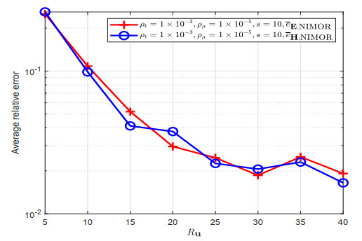
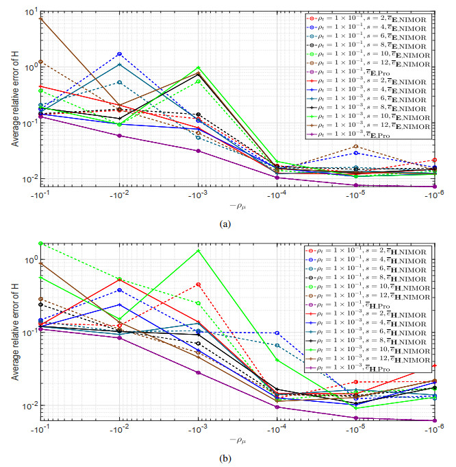
During the offline stage, the DGTD solver is utilized to acquire the HF solutions for $\mathcal{N}_p = 81$ training parameter values in the set $\mathcal{P}_{tr} = \{1, 1.05, 1.10, \cdots, 4.95, 5\}$ generated by uniform sampling between 1 and 5. The overall simulation duration is defined as 50 periods, which is equivalent to 50 m in normalized units with a time step $\Delta t$ = $3.678 \times 10^{-3}$ m. For each training parameter, the training snapshots are uniformly sampled from 49 m to 49.7 m in the set $\mathcal{T}_{tr} = \{49.0024 \text{ m}, 49.006 \text{ m}, \cdots, 49.6938 \text{ m}, 49.6975 \text{ m}\}$. The testing parameter set $\mathcal{P}_{test}$, consisting of 40 parameters generated by the LHS method, and the testing time set $\mathcal{T}_{test}$ with $\mathcal{N}_t = 263$ time points, covering the last period $\mathcal{T}_{test} = \mathcal{T}_{tr} \cup \{49.7012 \text{ m}, \ldots, 49.966 \text{ m}\}$, are employed to assess the proposed method. Due to the large dimensionality of the snapshots $\mathbf{S}_{\mathbf{u}}$, we employ a two-step POD method to extract the RB functions. When the truncation parameter is set to be $R_\mathbf{u} = 40$ in the CPD method, the convergence curves of the average relative error $\bar{e}_{\mathbf{u}, \mathrm{Pro}}$ and $\bar{e}_{\mathbf{u}, \text{NIMOR}}$ along with the truncation tolerances ($\rho_{t}, \rho_{\mu})$ and the time-delay parameter $s$ are plotted in Figure 1.

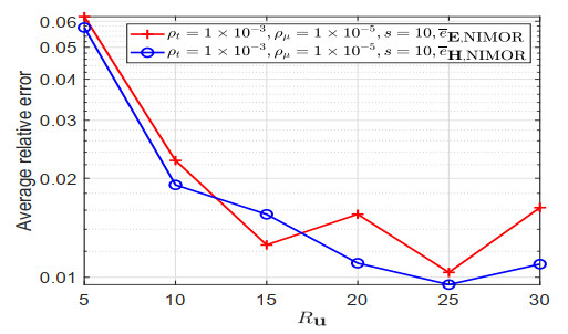
Combining Figures 1a,b, one can choose $s = 10$ for the HODMD method, and select $\rho_t = 1\times10^{-3}$, $\rho_\mu = 1\times10^{-5}$ in the two-step POD method to extract a set of $L_{H_x} = 139, L_{H_y} = 21$, and $L_{E_z} = 22$ RB functions. The NIMOR average relative error $\bar{e}_{\mathbf{u}, \text{NIMOR}}$ for different truncation parameters $R_\mathbf{u}$ are displayed on Figure 2.

The corresponding projection and NIMOR errors for $R_\mathbf{u} = 40$, $\rho_t = 1\times10^{-3}$, $\rho_\mu = 1\times10^{-5}$, and $s = 10$ are shown in Table 1.

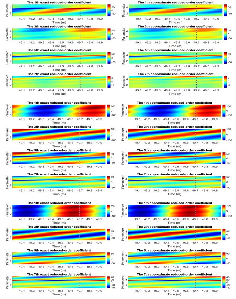
The approximate reduced-order coefficients and the corresponding exact values are shown in Figure 3. By comparison, the HODMD method performs very well in the prediction.

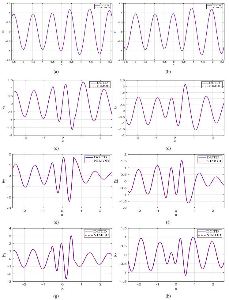
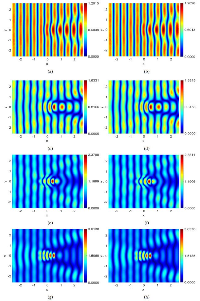
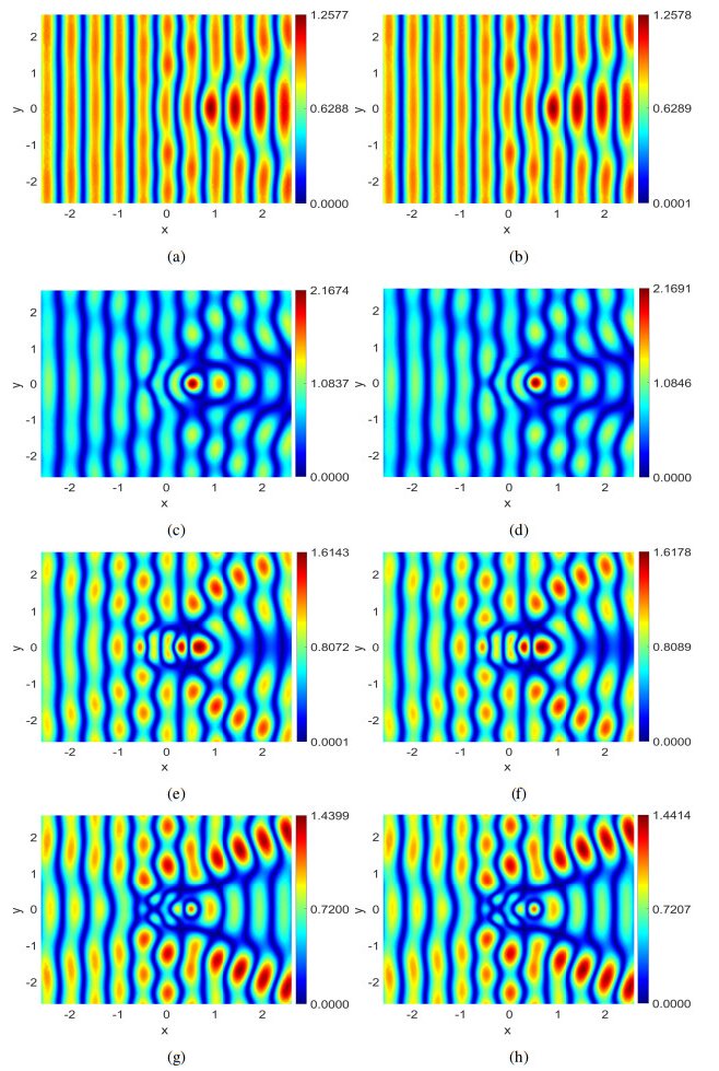
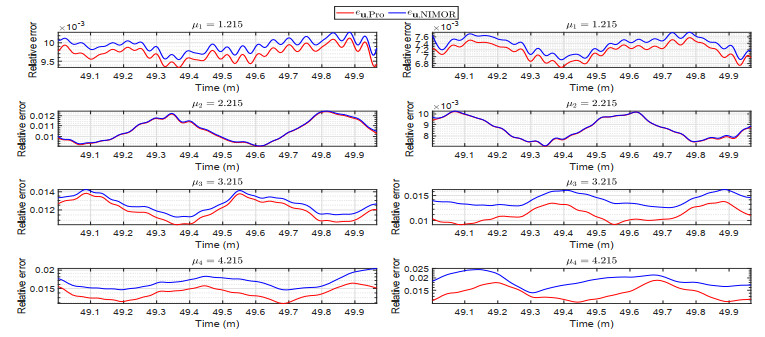
During the online stage, the reduced-order solutions at some selected testing parameters $\mu_{1} = 1.215$, $\mu_{2} = 2.215$, $\mu_{3} = 3.215$, and $\mu_{4} = 4.215$ are computed to assess the performance of the NIMOR method. To observe the visual effects of the electromagnetic field in the Fourier domain during the last oscillation period of the incident wave, we display the 1-D x-wise appearance of the real part of $E_z$ and $H_y$ along $y = 0$ in Figure 4, and their 2-D distributions in Figures 5 and 6. It can be observed that the reduced-order solutions match the DGTD solutions very well. Figure 7 shows the time evolution of the relative errors $e_{\mathbf{u}, \operatorname{Pro}}$ and $e_{\mathbf{u}, \operatorname{NIMOR}}$ for the four testing parameters in the testing time region $\mathcal{T}_{test}$. The computing time of the offline stage and the comparison between the online stage and the DGTD method are shown in Tables 2 and 3.

5.2.   Scattering of a plane wave by a multilayer disk

Next, we consider a high-dimensional parameter problem in the case of the scattering of a plane wave by a multilayer disk. The computation domain is the square $\Omega = [-3.2, 3.2] \times[-3.2, 3.2]$. The radius of each layer of the multilayer disk and the relative permeability are presented in Table 4.

The medium exterior of the multilayer disk is still assumed to be a vacuum. The range of the relative permittivity is formed as $\mu = (\varepsilon_{r, 1}, \varepsilon_{r, 2}, \varepsilon_{r, 3}, \varepsilon_{r, 4})\in\mathcal{P}$.

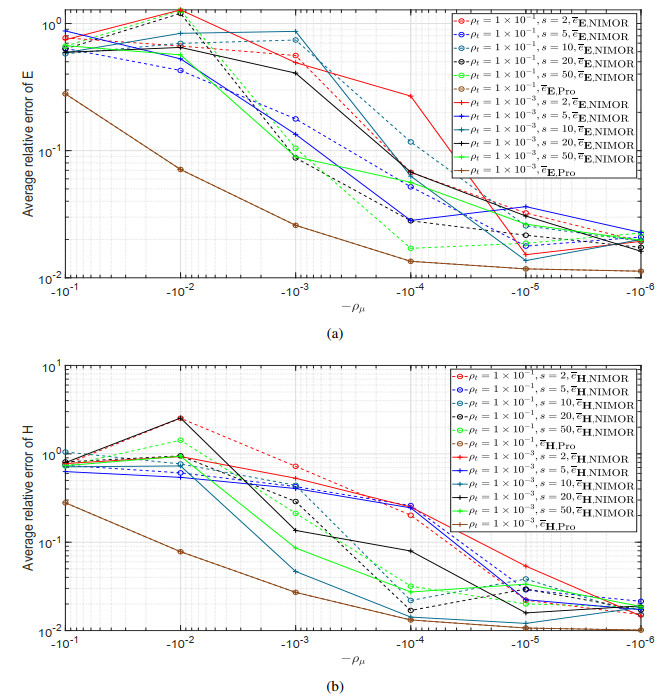
During the offline stage, the HF solutions are generated in a training parameter set $\mathcal{P}_{tr}$ chosen by the Smolyak sparse grid method with an approximation level of $L = 3$. The simulation duration is also 50 m with a time step $\Delta t$ = $3.800 \times 10^{-3}$ m. For each training parameter, the training snapshot vectors are uniformly sampled from 49 m to 49.7 m with the training time set $\mathcal{T}_{tr} = \{49.000 \text{ m}, 49.004 \text{ m}, \ldots, 49.6945\text{ m}, 49.6984 \text{ m}\}$. The testing parameter set $\mathcal{P}_{test}$, consisting of 81 parameters generated by the LHS method, and the testing time set $\mathcal{T}_{test}$ with $\mathcal{N}_t =$ 254 time points, covering the last period $\mathcal{T}_{test} = \mathcal{T}_{tr}\cup \{49.7012 \text{ m}, \ldots, 49.966 \text{ m}\}$, are employed to assess the proposed method. When the truncation parameter is set to be $R_\mathbf{u} = 20$, Figure 8 shows the convergence curves of the average relative error $\bar{e}_{\mathbf{u}, \mathrm{Pro}}$ and $\bar{e}_{\mathbf{u}, \text{NIMOR}}$ along with the truncation tolerances ($\rho_{t}, \rho_{\mu})$ and the time-delay parameter $s$.

Combining Figures 8a,b, one can choose $\rho_{t} = 1\times10^{-3}$ and $\rho_{\mu} = 1\times10^{-5}$. With the truncation tolerances $\rho_{t} = 1\times10^{-3}$ and $\rho_{\mu} = 1\times10^{-5}$, the reduced basis functions composed by a set of $L_{H_x} = 16$, $L_{H_y} = 15$, and $L_{E_z} = 15$ are extracted in the two-step POD method. Figure 9 shows the NIMOR average relative error $\bar{e}_{\mathbf{u}, \text{NIMOR}}$ for different truncation parameters in the CPD, and one can choose $R_\mathbf{u} = 25$. The corresponding average projection and NIMOR errors are displayed on the testing set in Table 5. Some approximate reduced-order coefficients and their corresponding exact values, both within the testing time set $\mathcal{T}_{test}$ and the training parameter set $\mathcal{P}_{tr}$, are shown in Figure 10.

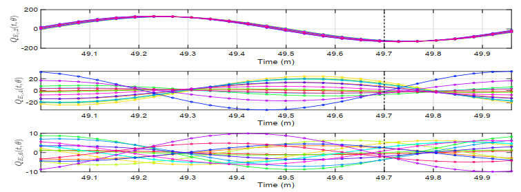
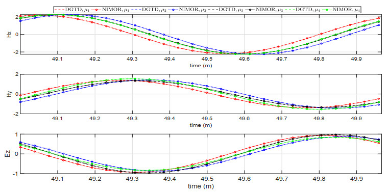
The reduced-order solutions at four testing parameters $\mu_{1} = \{5.125, 3.375, 2.125, 1.375\}$, $\mu_{2}\! = \!\{5.425, 3.625, 2.425, 1.625\}$, $\mu_{3}\! = \!\{5.125, 3.625, 2.125, 1.625\}$, $\mu_{4}\! = \!\{5.425, 3.375, 2.425, 1.375\}$ are computed to assess the performance of the NIMOR method during the online stage. The time evolution solutions of the NIMOR method and the DGTD method are shown in Figure 11.

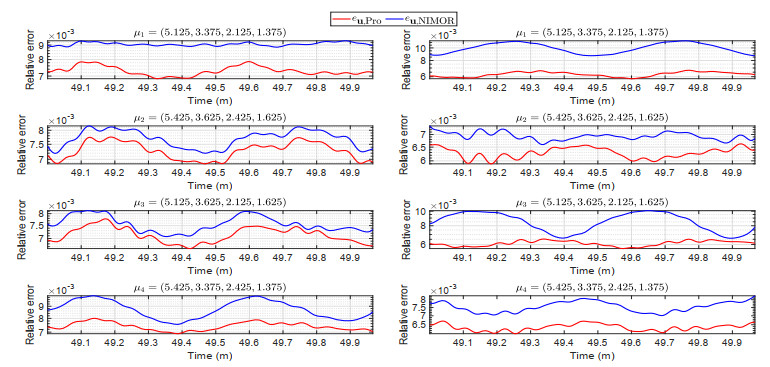
The time evolution of the relative errors $e_{\mathbf{u}, \operatorname{Pro}}$ and $e_{\mathbf{u}, \operatorname{NIMOR}}$ for the four testing parameters in the testing time region $\mathcal{T}_{test}$ are displayed in Figure 12.

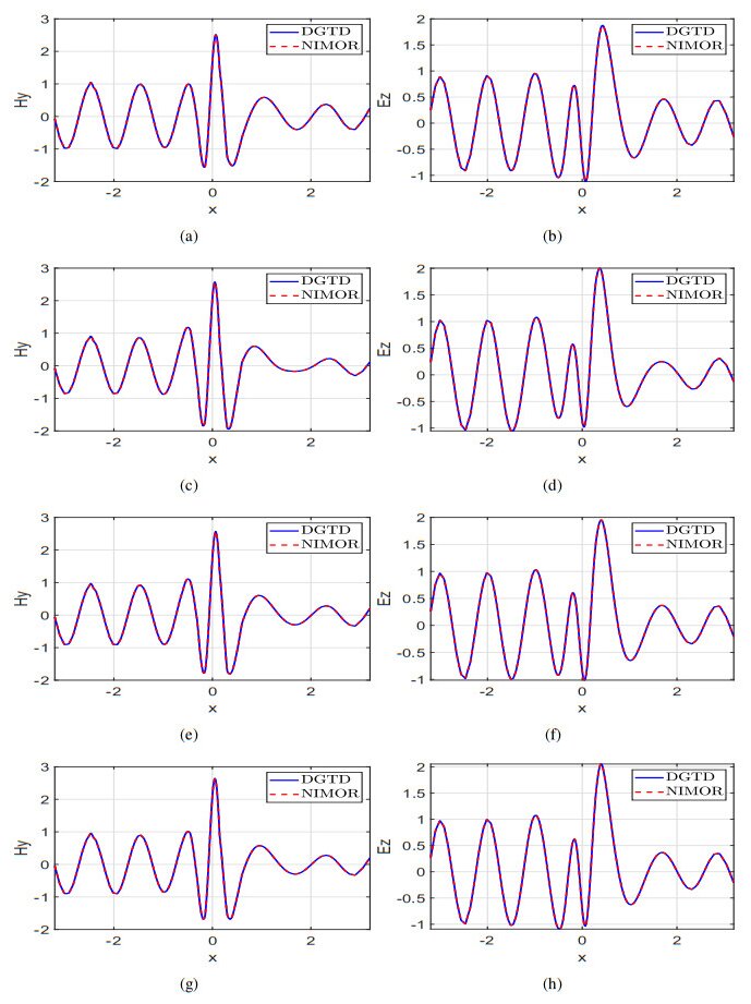
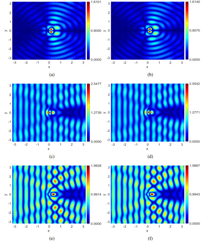
We display the 1-D x-wise appearance of the real part of $H_y$ and $E_z$ along $y = 0$ in Figure 13. The 2-D distribution of $H_x, H_y, E_z$ for $\mu_{2} = \{5.425, 3.625, 2.425, 1.625\}$ is shown in Figure 14.

The computing time of the offline stage and the comparison between the online stage and the DGTD method are shown in Tables 6 and 7.

6.   Conclusion

This work introduces a data-driven surrogate modeling approach that integrates the two-step POD, HODMD, and CPD methods for parameterized time-domain Maxwell's equations. During the offline stage, a set of RB functions are derived by the two-step POD method from HF solutions or snapshots. The HODMD method is then applied to predict the projection coefficients. The corresponding predicted coefficients are organized into a three-dimensional tensor, which is decomposed into time- and parameter-dependent components by the CPD method. Finally, the GPR method is used to approximate the relationship between the time/parameter values and the above components. During the online stage, the approximate solutions at some new time and parameter values can be quickly estimated. The accuracy and effectiveness of the NIMOR method are illustrated numerically, focusing on the scattering of a plane wave by a dielectric disk and by a multilayer heterogeneous medium. In the near future, more complex 3-D realistic applications, more generalization ability ^[37], and more precise parameter interpolation ^[38] may be considered.

Author contributions

Mengjun Yu: Investigation, Methodology, Writing, Software, Validation; Kun Li: Methodology, Validation, Writing, Supervision, Funding acquisition.

Use of AI tools declaration

The authors declare they have not used Artificial Intelligence (AI) tools in the creation of this article.

Acknowledgments

This research was supported by the Natural Science Foundation of Sichuan Province (Grant No. 24NSFSC1366).

Conflict of interest

The authors declare there is no conflict of interest.